TOC
Open TOC
Info
https://sites.cs.ucsb.edu/~lingqi/teaching/games101.html
https://www.bilibili.com/video/av90798049
计算机图形学概述
课程概述
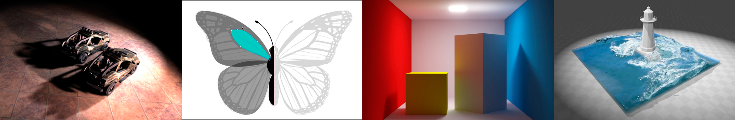
- Rasterization
Gold standard in Video Games (Real-time Applications)
- Curves and Meshes
- Ray Tracing
Gold standard in Animations / Movies (Offline Applications)
- Animation / Simulation
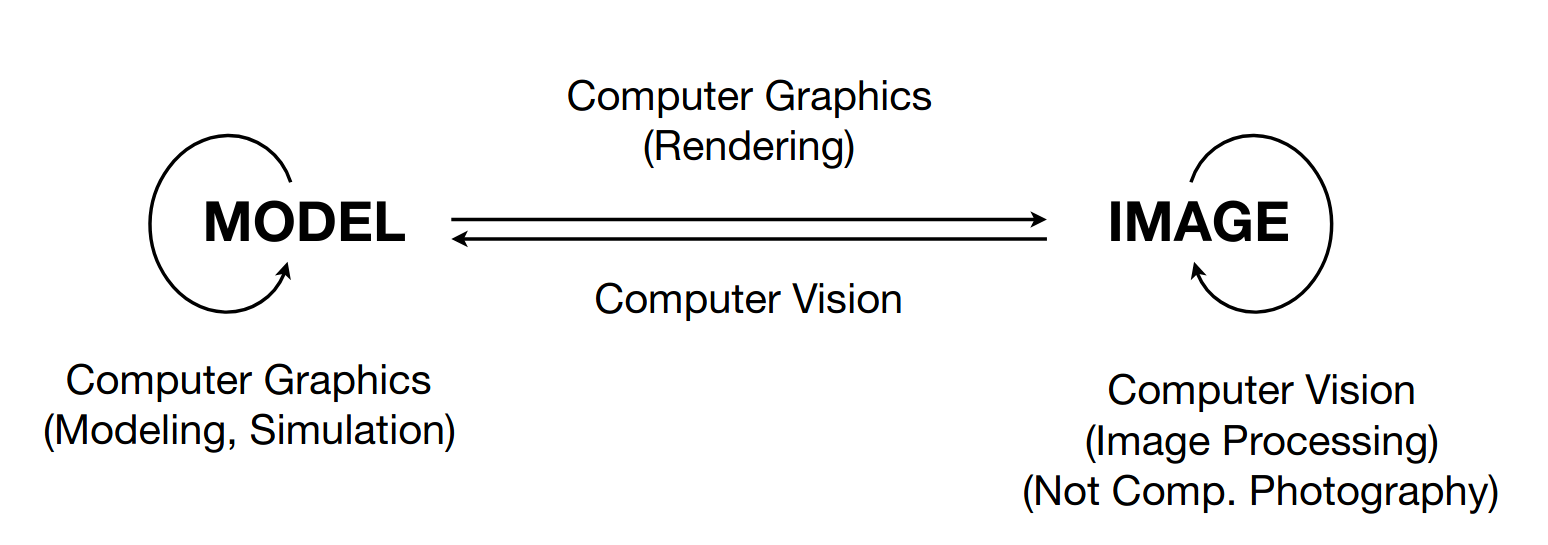
计算机图形学和计算机视觉
No clear boundaries.
向量与线性代数
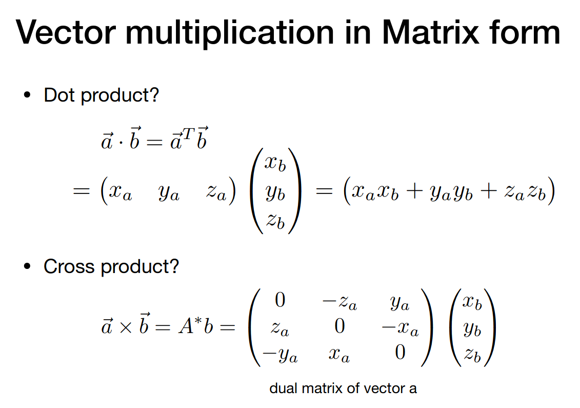
内积
Forward / backward (dot product positive / negative)
外积
Left / right (cross product outward / inward)
右手系
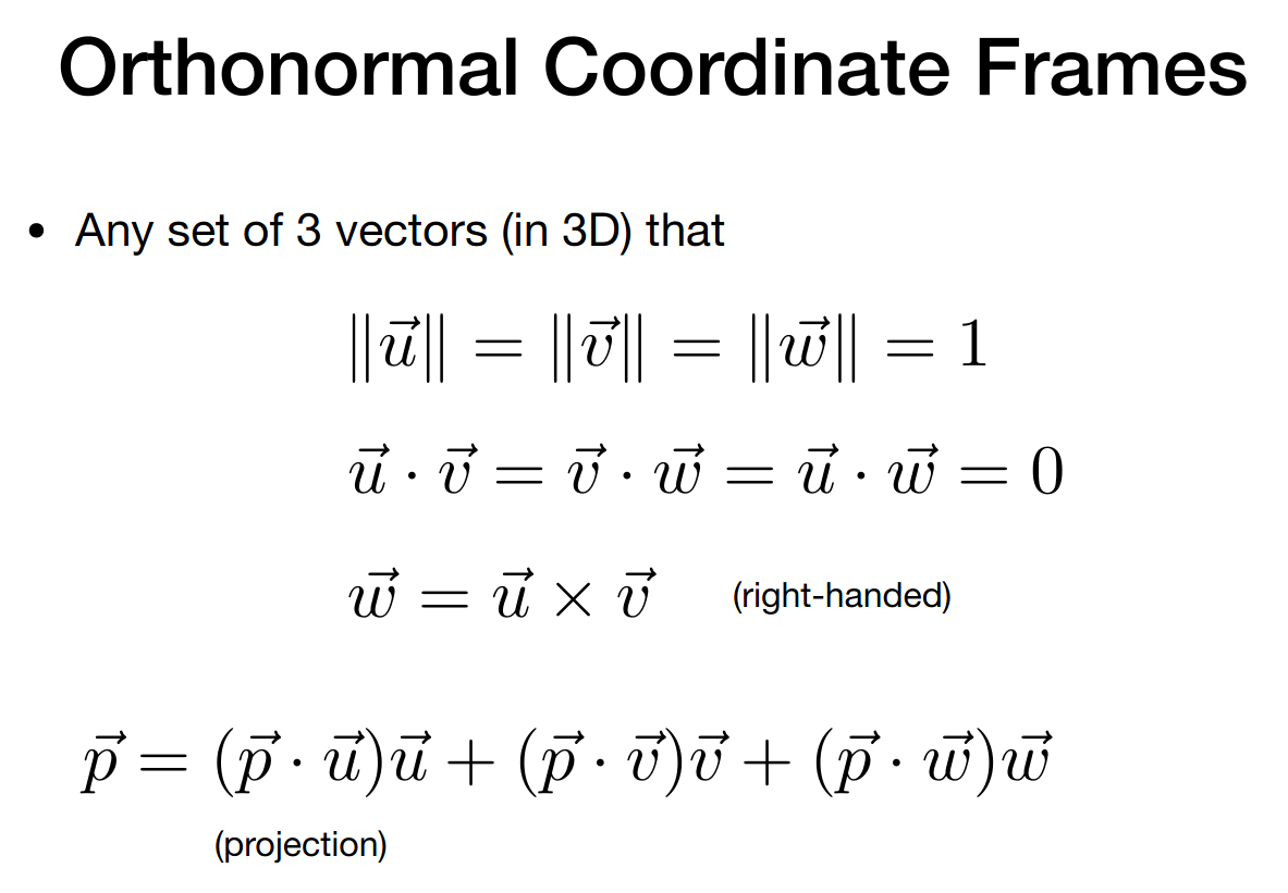
标准正交基
矩阵
变换(二维与三维)
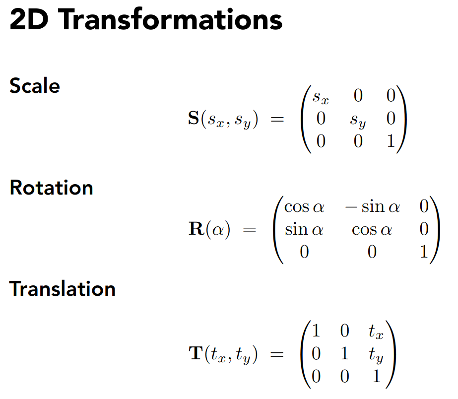
2D transformations
- Rotation
- 默认绕原点、逆时针方向
- Scale
- Shear
Homogeneous coordinates
注意到平移不是线性变换
于是引入齐次坐标形式,添加第三个分量
对于 point 而言
对于 vector 而言
基本的运算如下
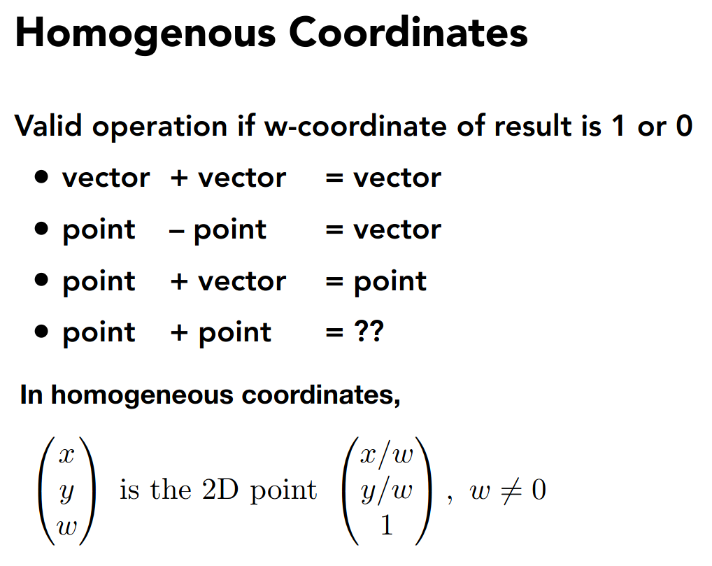
保持了相当的几何意义
注意 point 加上 point 定义为两个 point 的中点
于是对于仿射变换,可以统一为线性变换的形式
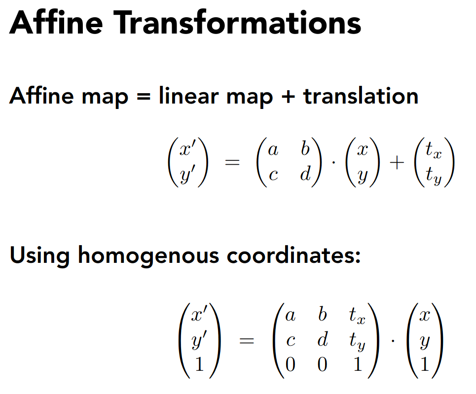
注意是先做线性变换,再做平移
于是统一了平移和线性变换
对于 3D Transformations,可以类似的推广
PA0
eigen
https://eigen.tuxfamily.org/index.php?title=Main_Page
sudo apt-get install libeigen3-devcmake
使用现代 cmake
cmake_minimum_required(VERSION 3.22.0)project(Transformation)
add_executable(Transformation main.cpp)
find_package(Eigen3 REQUIRED)target_include_directories(Transformation PUBLIC EIGEN3_INCLUDE_DIR)
target_link_libraries 似乎不必要
构建脚本 run.sh
rm -rf buildcmake -B build -DCMAKE_BUILD_TYPE=Debug -GNinjacmake --build build --target Transformationbuild/Transformationnote
简单的翻译一下即可
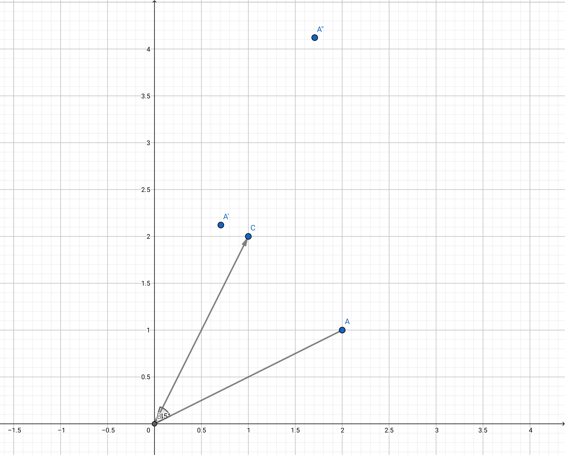
int main() {  const double pi = std::acos(-1);
  Eigen::Vector3f vec(2.0f, 1.0f, 1.0f);  Eigen::Matrix3f matrix;  matrix << std::cos(pi / 4), -std::sin(pi / 4), 1.0f, std::sin(pi / 4),      std::cos(pi / 4), 2.0f, 0.0f, 0.0f, 1.0f;
  std::cout << matrix * vec << std::endl;  return 0;}
输出为
1.707114.12132 1简单的验证一下
变换(模型、视图、投影)
3D Transformations
对于三维变换,有类似的齐次坐标形式
缩放和平移都十分 easy,下面考虑旋转
由于旋转的自由度变大了,先考虑简单的情形,即绕坐标轴旋转
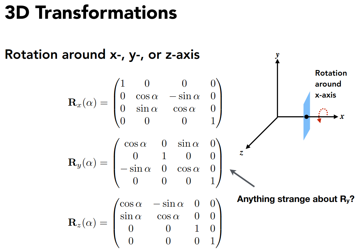
注意到
所以绕 y 轴旋转的矩阵有所不同
有了这三个矩阵,就可以描述三维空间中任意的旋转,这便是欧拉角
详见
另外还有一个公式叫罗德里格旋转公式
详见
Viewing transformation
想象在拍照片
- Find a good place and arrange people. (model transformation)
- Find a good angle to put the camera. (view transformation)
- Cheese! (projection transformation)
主要介绍后两种变换
View transformation
主要是摆放相机的位置
首先需要描述相机的位置
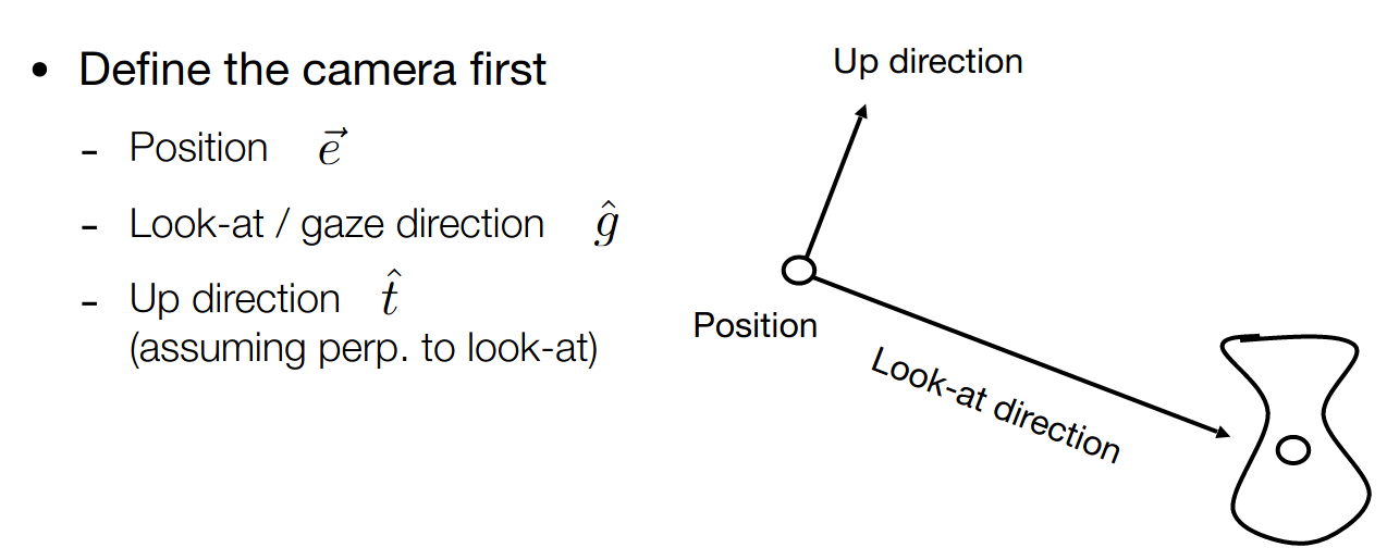
注意到物体和相机的相对位置
我们简化为,相机位于原点,头顶 y 轴,朝向 -z 轴,即
下面考虑如何将相机变换到这个位置,这样物体只要使用相同的变换,就能保证相对位置不变
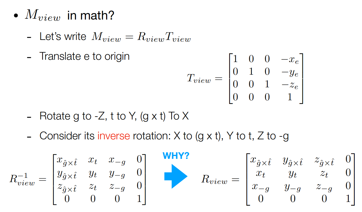
先做平移,再做旋转
第二步的关键在于,旋转变换矩阵是正交矩阵,即
所以可以考虑逆变换,即将坐标轴旋转到相应的位置
Projection transformation
分为正交投影和透视投影
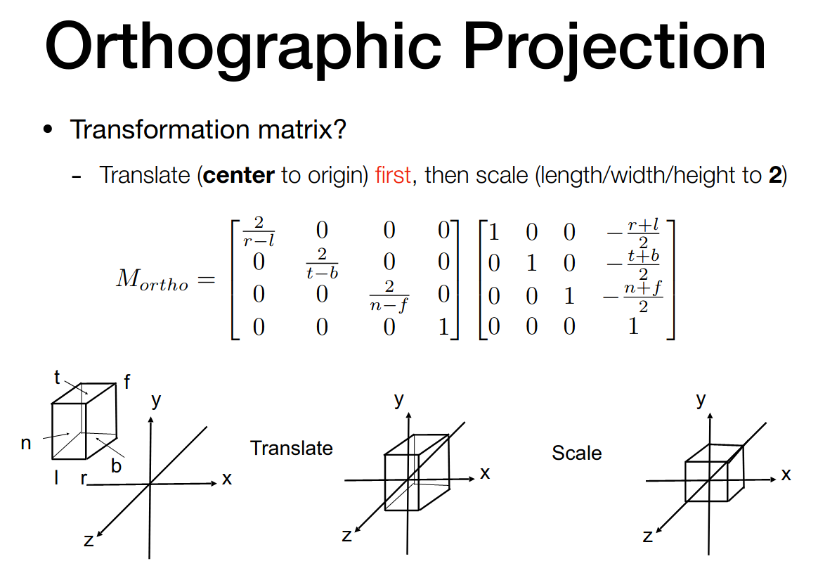
Orthographic Projection
We want to map a cuboid [l, r] x [b, t] x [f, n] to the canonical cube
left, right, bottom, top, far, near
由于相机朝向 -z 轴,所以 far 的 z 坐标更小
单位立方体就是
变换矩阵不难得到
Perspective Projection
使用化归的思想,先将台体变换为长方体,再使用正交投影
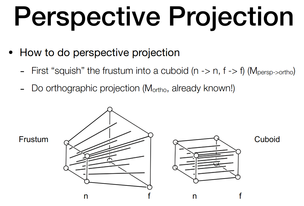
这里有一些假设
- near 平面不变
- far 平面的 z 坐标不变
- far 平面的中心点不变
根据相似三角形关系,可以得到 x 分量和 y 分量的变换关系
于是有
注意对齐次坐标中的 point 各分量数乘某个非零值并不改变 point
可以不严谨的得到
下面根据假设,取 near 平面上的某点,在变换后不变,即
取 far 平面的中心点,在变换后不变,即
综合诸式,可以不严谨的得到
再左乘正交投影的矩阵即可
**思考题:**对于 near 平面和 far 平面的中间平面,考虑其中心点
注意到
所以实际上会变远
光栅化(三角形的离散化)
Viewport transformation
接着上节课的内容
当得到了一个单位立方体后,我们需要将其绘制在屏幕上
为简化考虑,我们忽略 z 分量,并做如下的变换
这里的 width 和 height 是屏幕的参数
更具体的,屏幕实际上是像素的二维数组
而光栅化表示在屏幕上绘制像素
目前我们使用 RGB 表示像素
下面定义 screen space
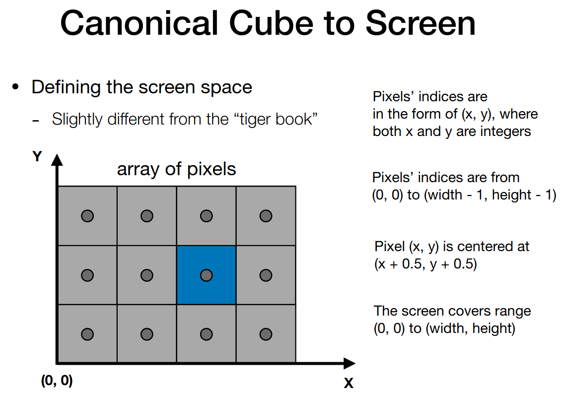
注意区分像素和像素的下标
如此,Viewport transform matrix 易得如下
Rasterization
Different raster displays
略
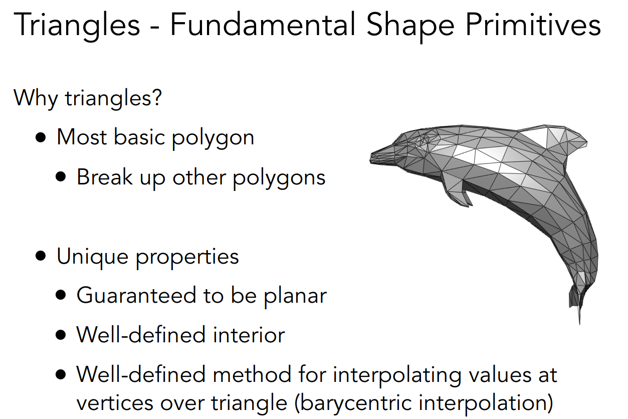
Rasterizing a triangle
绘制的基本单元为三角形,理由如下
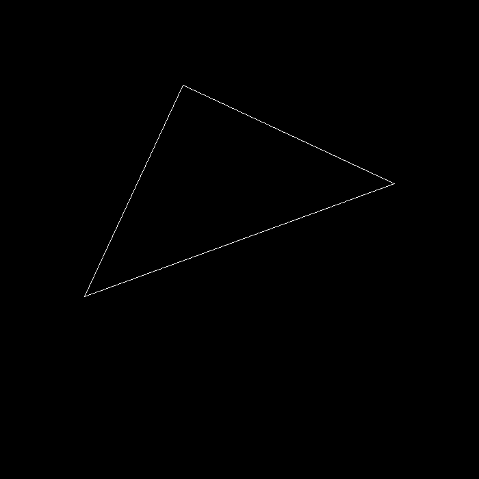
当我们得到三角形的三个顶点的坐标后,需要以像素的形式绘制出来
最基本的想法是——采样
使用一个二重循环即可
for (int x = 0; x < xmax; ++x) for (int y = 0; y < ymax; ++y) image[x][y] = inside(tri, x + 0.5, y + 0.5);注意像素的中心需要加上 0.5
而 inside 函数用来判断该像素是否在三角形内部
显然,我们需要使用外积
当下面三个式子同向时
P 点就在三角形内部
一些其他议题:
- Edge Cases
- 光栅化加速
- 抗锯齿
PA1
opencv
sudo apt install libopencv-dev python3-opencvrun
可以直接 ./run.sh,按 ESC 退出
也可以指定参数
./build/Rasterizer -r 20 pa1.pngmv pa1.png ~/Desktop/virtual-machine-repository/post/games101.assets/note
两个函数的实现是简单的
Eigen::Matrix4f get_model_matrix(float rotation_angle) {  Eigen::Matrix4f model = Eigen::Matrix4f::Identity();
  // TODO: Implement this function  // Create the model matrix for rotating the triangle around the Z axis.  // Then return it.  float radian = rotation_angle / 180 * MY_PI;
  Eigen::Matrix4f translate;  translate << std::cos(radian), -std::sin(radian), 0, 0, std::sin(radian),      std::cos(radian), 0, 0, 0, 0, 1, 0, 0, 0, 0, 1;
  model = translate * model;
  return model;}
Eigen::Matrix4f get_projection_matrix(float eye_fov, float aspect_ratio,                                      float zNear, float zFar) {  Eigen::Matrix4f projection = Eigen::Matrix4f::Identity();
  // TODO: Implement this function  // Create the projection matrix for the given parameters.  // Then return it.  float yTop = std::abs(zNear) * std::tan(eye_fov / 360 * MY_PI);  float xRight = yTop * aspect_ratio;
  Eigen::Matrix4f ortho;  ortho << 1 / xRight, 0, 0, 0, 0, 1 / yTop, 0, 0, 0, 0,      2 / std::abs(zFar - zNear), 0, 0, 0, 0, 1;  Eigen::Matrix4f persp;  persp << zNear, 0, 0, 0, 0, zNear, 0, 0, 0, 0, zNear + zFar, -zNear * zFar, 0,      0, 1, 0;
  projection = ortho * persp * projection;
  return projection;}
提高项需要使用罗德里格旋转公式,就不做了
先分析一下三个变换矩阵
- model
实际上就是绕 z 轴旋转
通过命令行指定 angle
也可以通过按 A 键与 D 键动态的变换 angle
- view
实际上就是移动相机的位置
使用 eye_pos 描述
Eigen::Vector3f eye_pos = {0, 0, 5};- projection
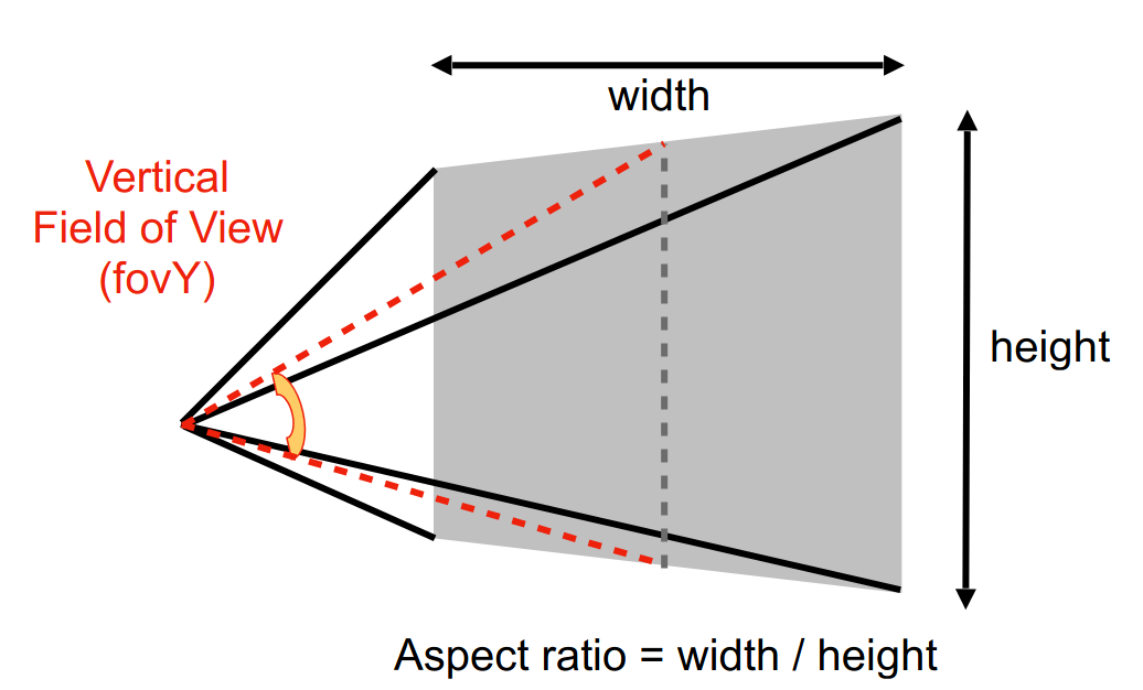
给出了 field-of-view (fov) 和 aspect ratio
有如下的关系
进而得到 left, right, bottom, top, far, near
需注意这里假定了对称性 l = -r, b = -t
然后先透视再正交投影即可
pic
修正透视投影矩阵后
光栅化(深度测试与抗锯齿)
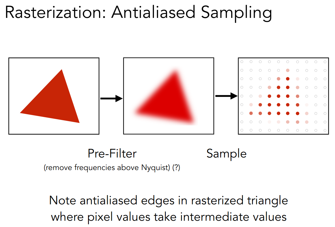
这一讲主要分析和处理 Aliasing Artifacts 问题
当采样频率低于实际信号的频率时,就会出现 Aliasing Artifacts
而一种解决方案就是进行 Pre-Filter 后,再进行 Sample
注意顺序
下面解释
- Why undersampling introduces aliasing?
- Why pre-filtering then sampling can do antialiasing?
Why undersampling introduces aliasing?
从 spatial domain 和 frequency domain 两个角度来理解
祭出傅里叶变换
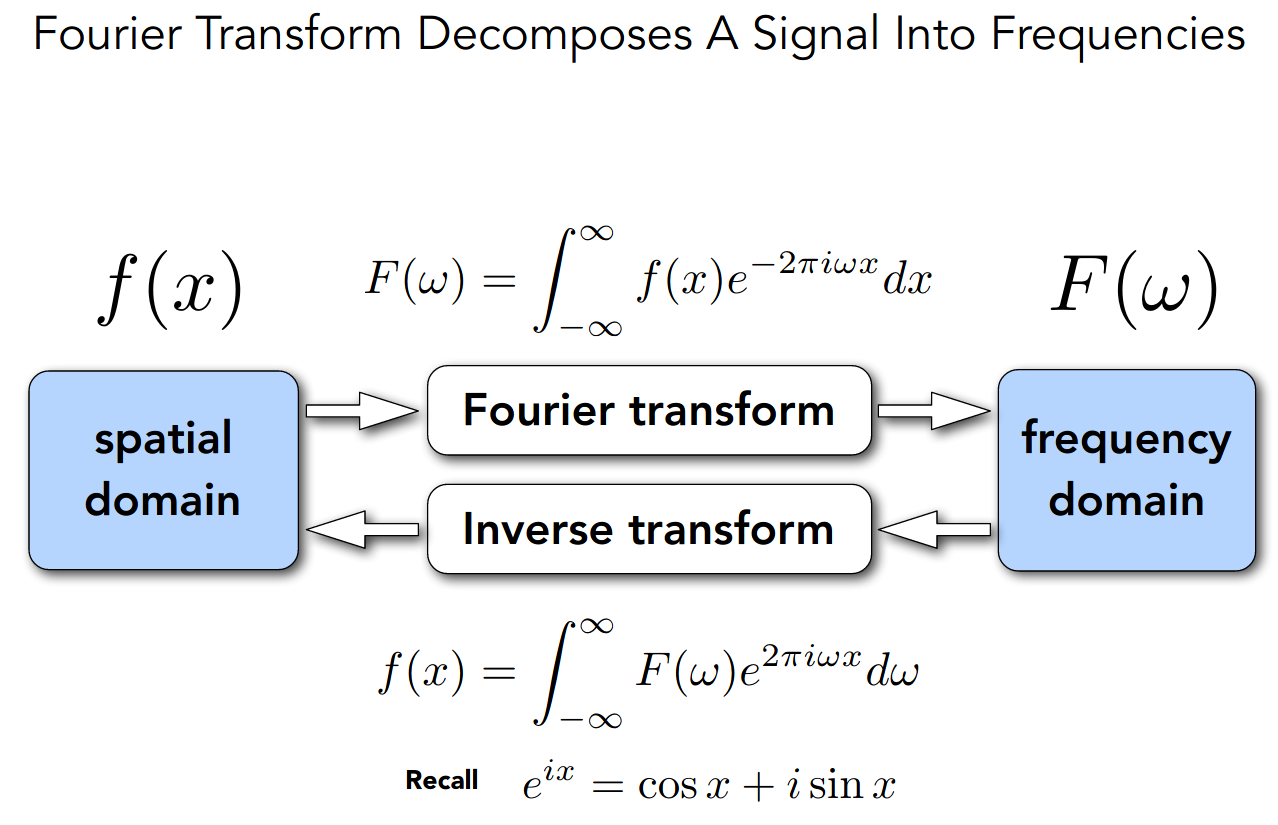
从 spatial domain 来理解
从 frequency domain 来理解
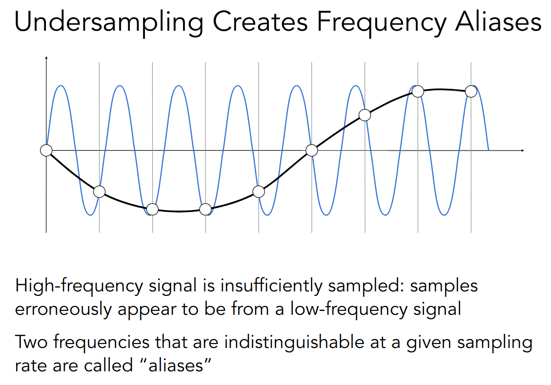
- Sampling = Repeating Frequency Contents
- Aliasing = Mixed Frequency Contents
这里似乎有关系,采样频率越低,在 spatial domain 间隔越大,在 frequency domain 间隔越小
具体见课件,反正不太懂
Why pre-filtering then sampling can do antialiasing?
在无法提升采样频率的前提下,使用低通滤波器过滤高频信息,可以避免 Mixed Frequency Contents
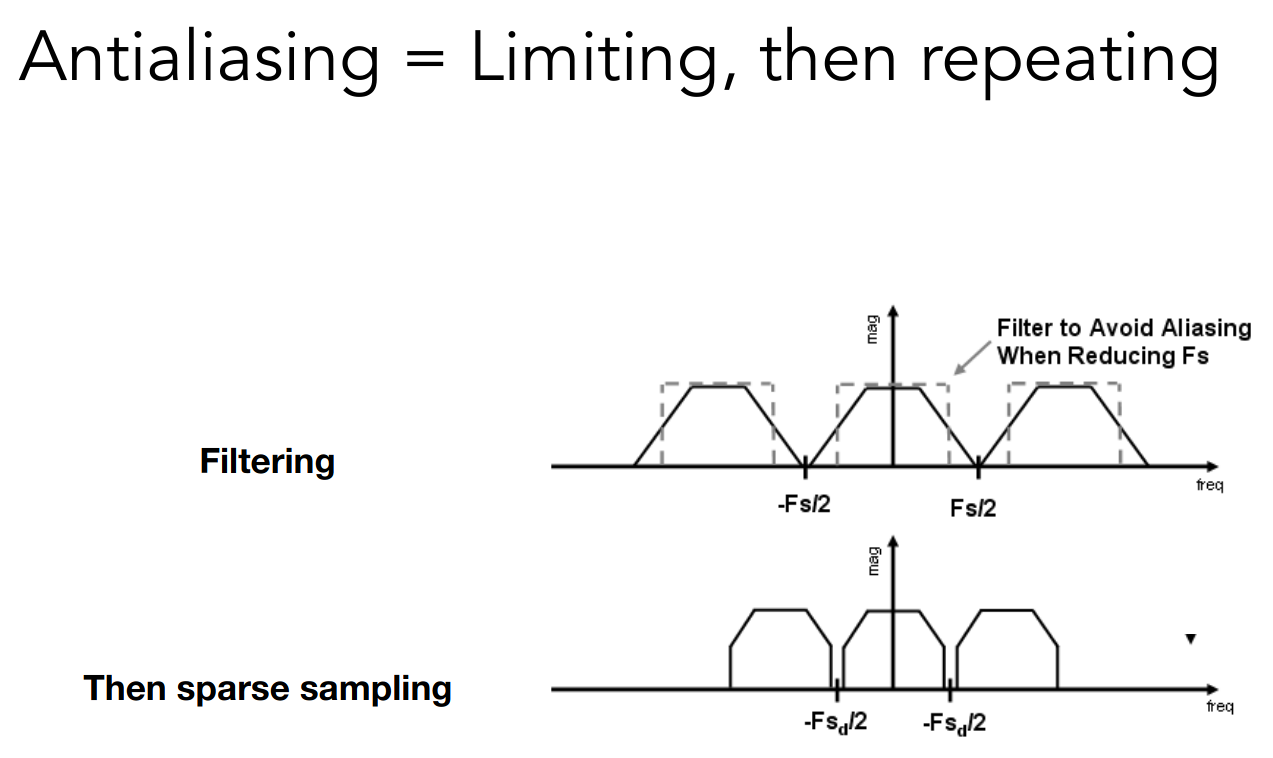
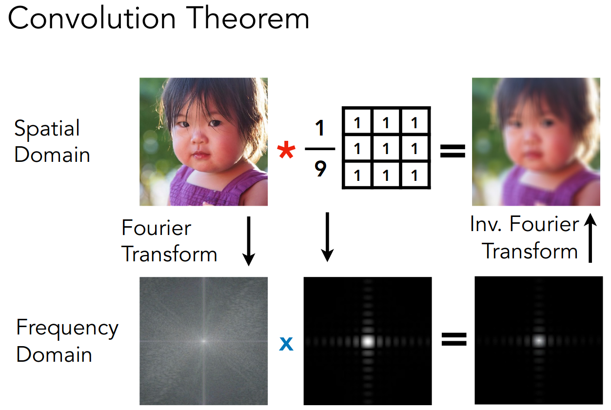
而过滤,在 spatial domain 中就是卷积,就是取平均值,在 frequency domain 中就是相乘
Antialiasing in practice
以此为基础,有如下解决 Aliasing Artifacts 的方案
- 提升采样率
- 也就是更大的屏幕
- MSAA
- 多重采样取均值
- 注意这并没有提升采样率

其他技术
- FXAA (Fast Approximate AA)
- TAA (Temporal AA)
- Super resolution / super sampling
- DLSS (Deep Learning Super Sampling)
着色(光照与基本着色模型)
Z-buffering
光栅化最后的内容
主要解决 visibility / occlusion 的问题
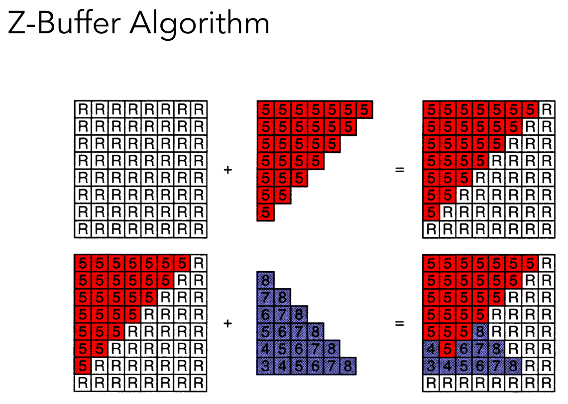
思想如下
- Store current min. z-value for each sample (pixel)
- Needs an additional buffer for depth values
- frame buffer stores color values
- depth buffer (z-buffer) stores depth
算法伪代码如下
for (each triangle T) for (each sample (x,y,z) in T) if (z < zbuffer[x,y]) // closest sample so far framebuffer[x,y] = rgb; // update color zbuffer[x,y] = z; // update depth else ; // do nothing, this sample is occluded两个注意点
- 为了方便处理,我们将 z 进行了反转,保证都是正数,并且越大表示离视点越远
- 若不使用抗锯齿,就是以像素为单位,否则可能以采样点为单位
一个简单的例子
若每个三角形占据常数个像素,算法复杂度与三角形个数成线性关系
Shading
我们给着色一个定义
- In Merriam-Webster Dictionary
The darkening or coloring of an illustration or diagram with parallel lines or a block of color.
- In this course
The process of applying a material to an object.
下面考虑一个简单的着色模型
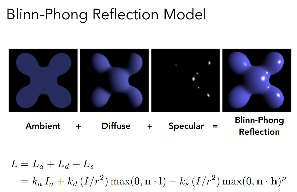
Blinn-Phong Reflectance Model
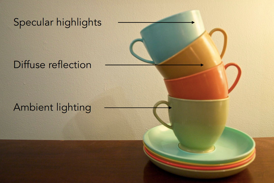
从上到下依次为
- 高光
- 漫反射
- 环境光
需要给着色点进行形式化描述
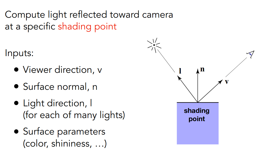
也就是考虑观察方向,光线方向和表面的法向
均为单位向量
需要注意着色具有局部性(近似为平面才有法向),因而不会因为光线的遮挡而产生阴影
shading ≠ shadow
下面给出漫反射的一个近似公式

注意里面的 I 为光能,r 代表光源和着色点的距离
通过球壳表面光能固定推导出平方反比的关系
而 k 是材质与漫反射相关的系数
注意对于漫反射而言,无论观察方向,着色都是一致的
PA2
color
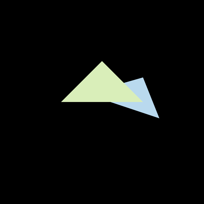
三角形一
三角形二
run
可以这样指定参数
./build/Rasterizer pa2.pngmv pa2.png ~/Desktop/virtual-machine-repository/post/games101.assets/note
// Screen space rasterizationvoid rst::rasterizer::rasterize_triangle(const Triangle &t) {  auto v = t.toVector4();
  // TODO : Find out the bounding box of current triangle.  // iterate through the pixel and find if the current pixel is inside the  // triangle  int xmin = std::floor(std::min(t.v[0].x(), std::min(t.v[1].x(), t.v[2].x())));  int xmax = std::ceil(std::max(t.v[0].x(), std::max(t.v[1].x(), t.v[2].x())));  int ymin = std::floor(std::min(t.v[0].y(), std::min(t.v[1].y(), t.v[2].y())));  int ymax = std::ceil(std::max(t.v[0].y(), std::max(t.v[1].y(), t.v[2].y())));
  for (int i = xmin; i <= xmax; ++i) {    for (int j = ymin; j <= ymax; ++j) {      float x = i + 0.5;      float y = j + 0.5;
      if (insideTriangle(x, y, t.v)) {        // If so, use the following code to get the interpolated z value.        auto [alpha, beta, gamma] = computeBarycentric2D(x, y, t.v);        float w_reciprocal =            1.0 / (alpha / v[0].w() + beta / v[1].w() + gamma / v[2].w());        float z_interpolated = alpha * v[0].z() / v[0].w() +                               beta * v[1].z() / v[1].w() +                               gamma * v[2].z() / v[2].w();        z_interpolated *= w_reciprocal;
        // TODO : set the current pixel (use the set_pixel function) to the        // color of        // the triangle (use getColor function) if it should be painted.        if (-z_interpolated < depth_buf[get_index(i, j)]) {          depth_buf[get_index(i, j)] = -z_interpolated;          frame_buf[get_index(i, j)] = t.getColor();        }      }    }  }}
先创建 bounding box
然后遍历每个像素,注意像素中心的屏幕空间坐标需要加上 0.5
使用 insideTriangle 判断是否在三角形内部
static bool insideTriangle(float x, float y, const Vector3f *_v) {  // TODO : Implement this function to check if the point (x, y) is inside the  // triangle represented by _v[0], _v[1], _v[2]  Eigen::Vector3f ab(_v[0].x() - _v[1].x(), _v[0].y() - _v[1].y(), _v[0].z() - _v[1].z());  Eigen::Vector3f bc(_v[1].x() - _v[2].x(), _v[1].y() - _v[2].y(), _v[1].z() - _v[2].z());  Eigen::Vector3f ca(_v[2].x() - _v[0].x(), _v[2].y() - _v[0].y(), _v[2].z() - _v[0].z());
  Eigen::Vector3f au(_v[0].x() - x, _v[0].y() - y, _v[0].z() - 0);  Eigen::Vector3f bu(_v[1].x() - x, _v[1].y() - y, _v[1].z() - 0);  Eigen::Vector3f cu(_v[2].x() - x, _v[2].y() - y, _v[2].z() - 0);
  auto res1 = ab.cross(au).z();  auto res2 = bc.cross(bu).z();  auto res3 = ca.cross(cu).z();
  return (res1 > 0 && res2 > 0 && res3 > 0) ||         (res1 < 0 && res2 < 0 && res3 < 0);}
这里将参数改成了 float
使用三维向量进行外积,z 分量为 0
最后只要看外积出的向量的 z 分量即可
然后计算出插值深度值,并与深度缓冲区中的相应值进行比较
这里奇怪的是需要对插值深度值取负,否则深度关系就反了
感觉哪里实现错了
最后更新 depth_buf 和 frame_buf 即可
使用 get_index 函数将二维坐标转换为一维坐标
后来发现是透视投影矩阵有点问题
由于传入 get_projection_matrix 函数的 zNear 和 zFar 是正数
所以实际上要将透视投影矩阵的 n 和 f 取负
简单的做法就是这样
这样的话就不需要对插值深度值取负了
pic
修正透视投影矩阵后
大小有点怪怪的

antialiasing
框架不变,只是在填充 frame_buf 时取平均
if (z_interpolated < depth_buf[get_index(i, j)]) { depth_buf[get_index(i, j)] = z_interpolated; int sum{}; sum += static_cast<int>(insideTriangle(x - 0.25, y - 0.25, t.v)); sum += static_cast<int>(insideTriangle(x - 0.25, y + 0.25, t.v)); sum += static_cast<int>(insideTriangle(x + 0.25, y - 0.25, t.v)); sum += static_cast<int>(insideTriangle(x + 0.25, y + 0.25, t.v)); frame_buf[get_index(i, j)] = t.getColor() * (sum / 4.0); }确实优化了一丢丢
着色(着色频率、图形管线、纹理映射)
Blinn-Phong reflectance model
接着上节课的内容
下面给出高光的一个近似公式
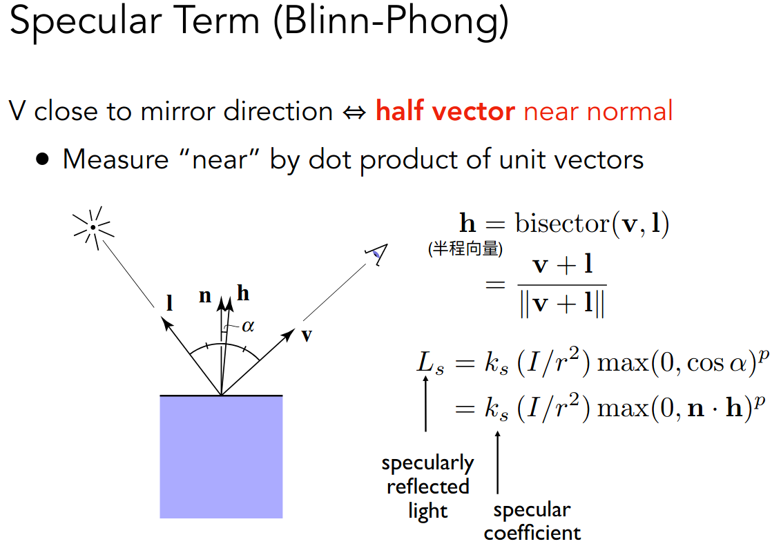
这里进行了一次转化,对于高光而言,可以近似认为是镜面反射,设反射光为 I’
那么有角度关系
也就是转化为半程向量和法向量之间的夹角
而常数 p 可以用来控制 reflection lobe
对于环境光而言,在固定光能和系数的情形下,可以认为是常数
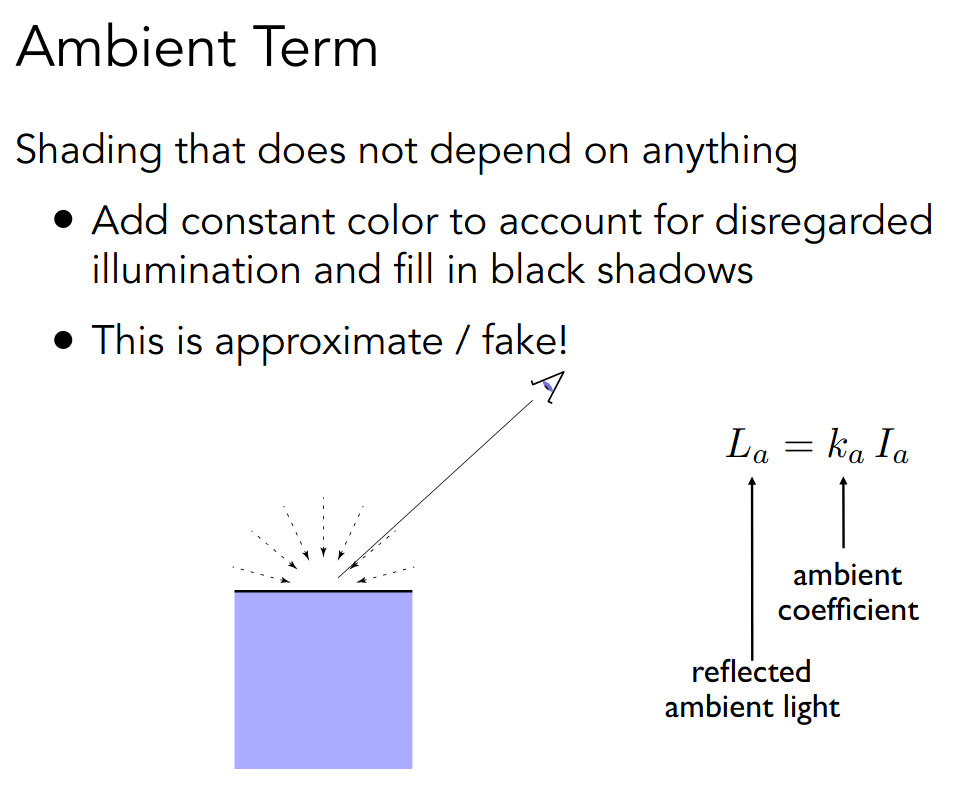
于是 Blinn-Phong Reflectance Model 总结如下
Shading Frequencies
一图胜千言
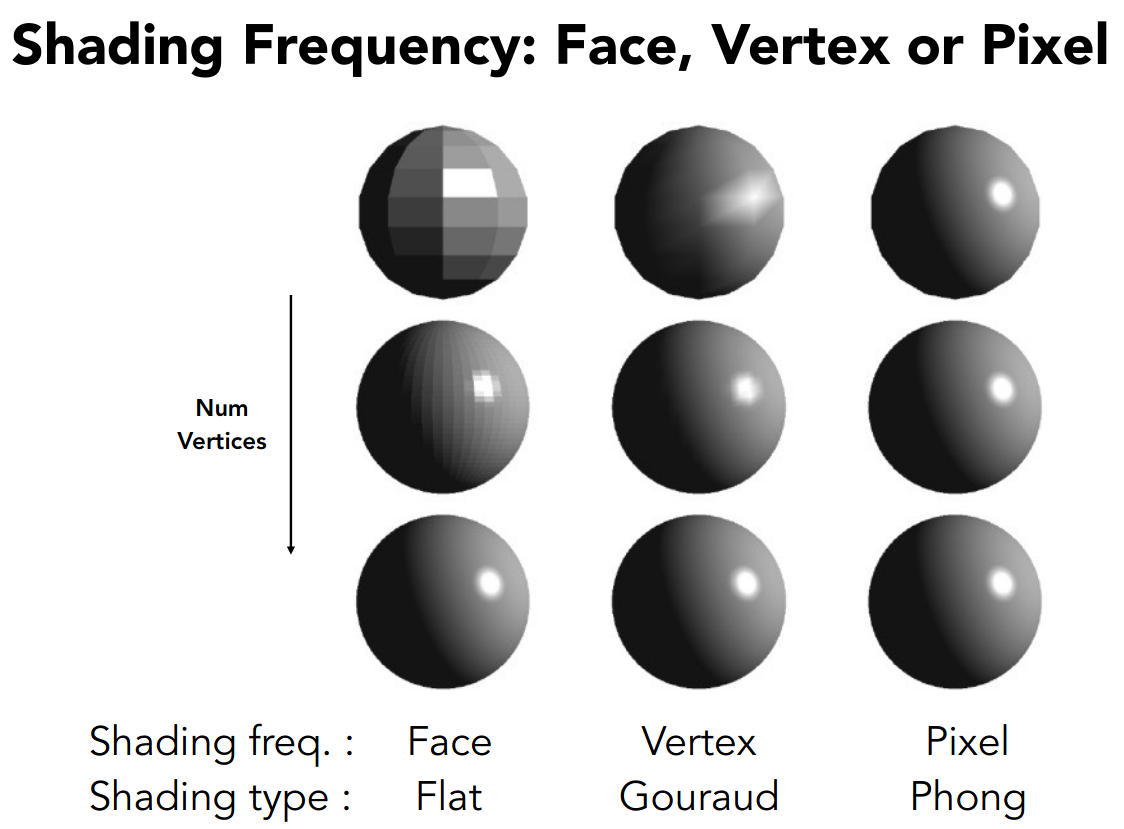
Flat 是每个三角形视为一个着色点
Gouraud 是每个三角形的顶点视为一个着色点,顶点的法向量通过对周围三角形的法向量取均值得到
Phong 是每个像素视为一个着色点,像素的法向量通过插值得到
Graphics (Real-time Rendering) Pipeline
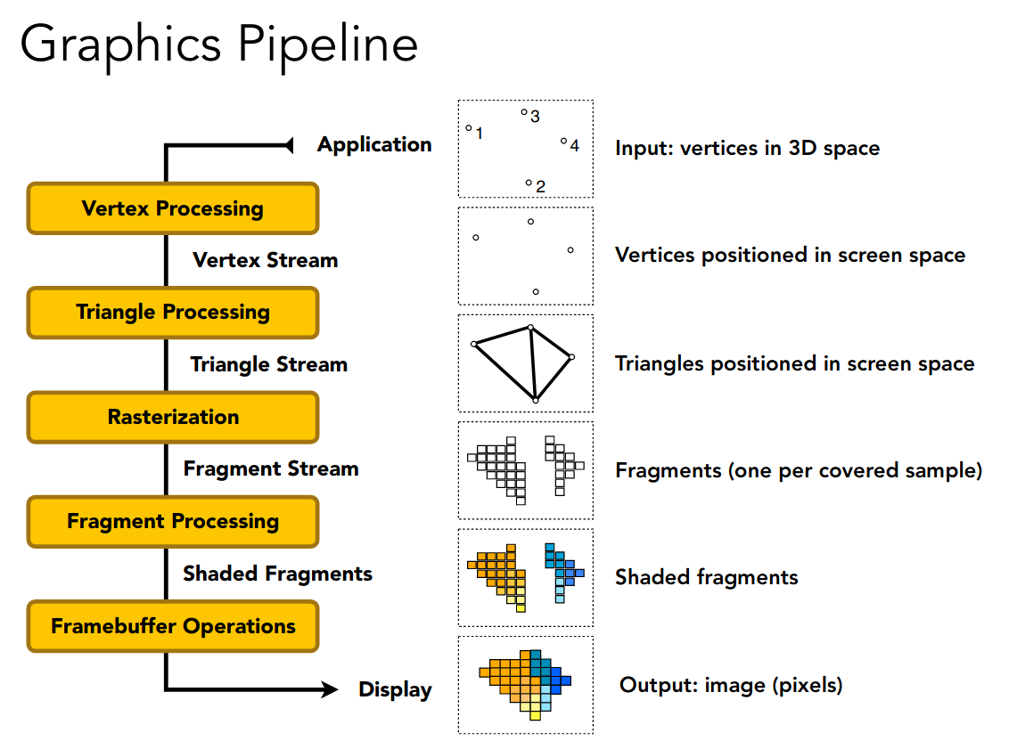
这里相当于总结了目前所学的内容
引入了顶点处理的步骤
从而着色可以选择在 Vertex Processing 中进行,着色频率为 Gouraud
也可以选择在 Fragment Processing 中进行,着色频率为 Phong 或 Flat
Shader Programs
着色器就是在某些阶段处理着色的程序
Example GLSL fragment shader program
uniform sampler2D myTexture; // program parameteruniform vec3 lightDir; // program parametervarying vec2 uv; // per fragment value (interp. by rasterizer)varying vec3 norm; // per fragment value (interp. by rasterizer)void diffuseShader(){ vec3 kd; kd = texture2d(myTexture, uv); // material color from texture kd *= clamp(dot(–lightDir, norm), 0.0, 1.0); // Lambertian shading model gl_FragColor = vec4(kd, 1.0); // output fragment color}描述了对单个顶点或像素进行的操作
另外推荐一个网站 https://www.shadertoy.com/
GPU
实现图形管线的硬件便是 GPU
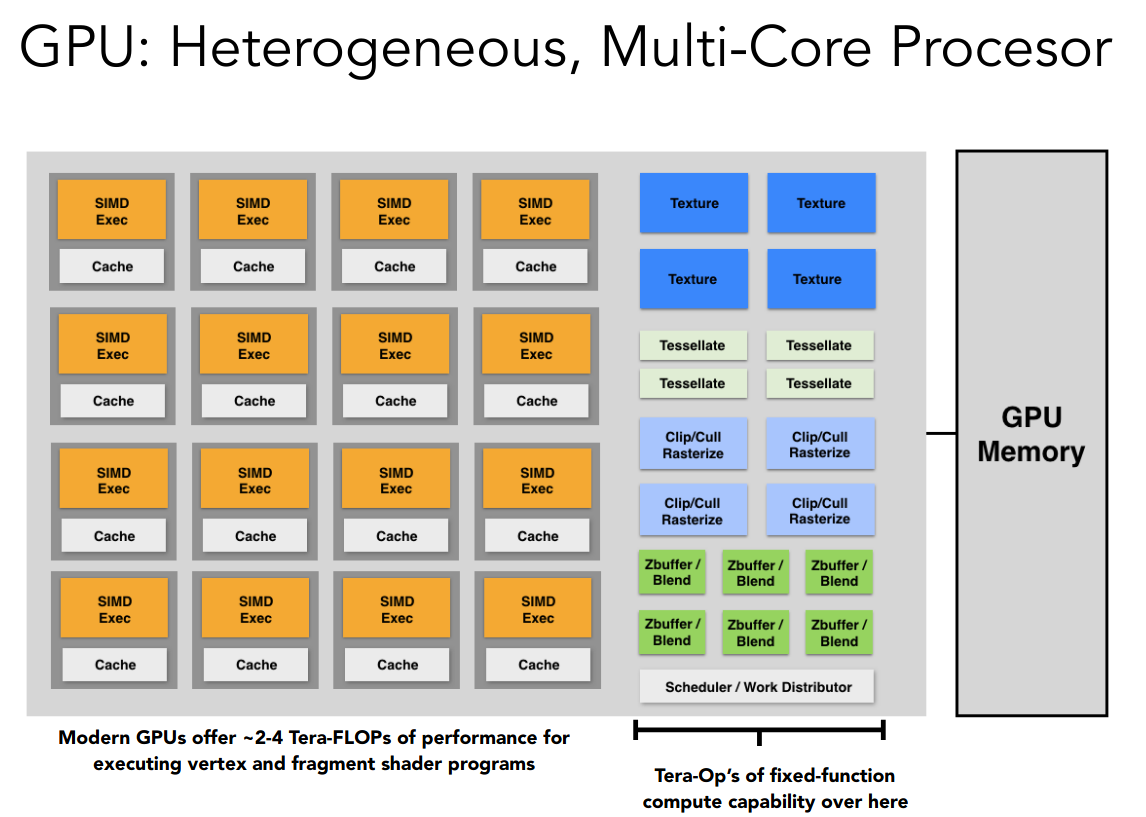
多核心,高度并行
Texture Mapping
独眼巨人警告
相当于从屏幕空间到纹理空间的映射
定义了 Blinn-Phong reflectance model 公式的中的 k 值
我们以漫反射的 k 值为例
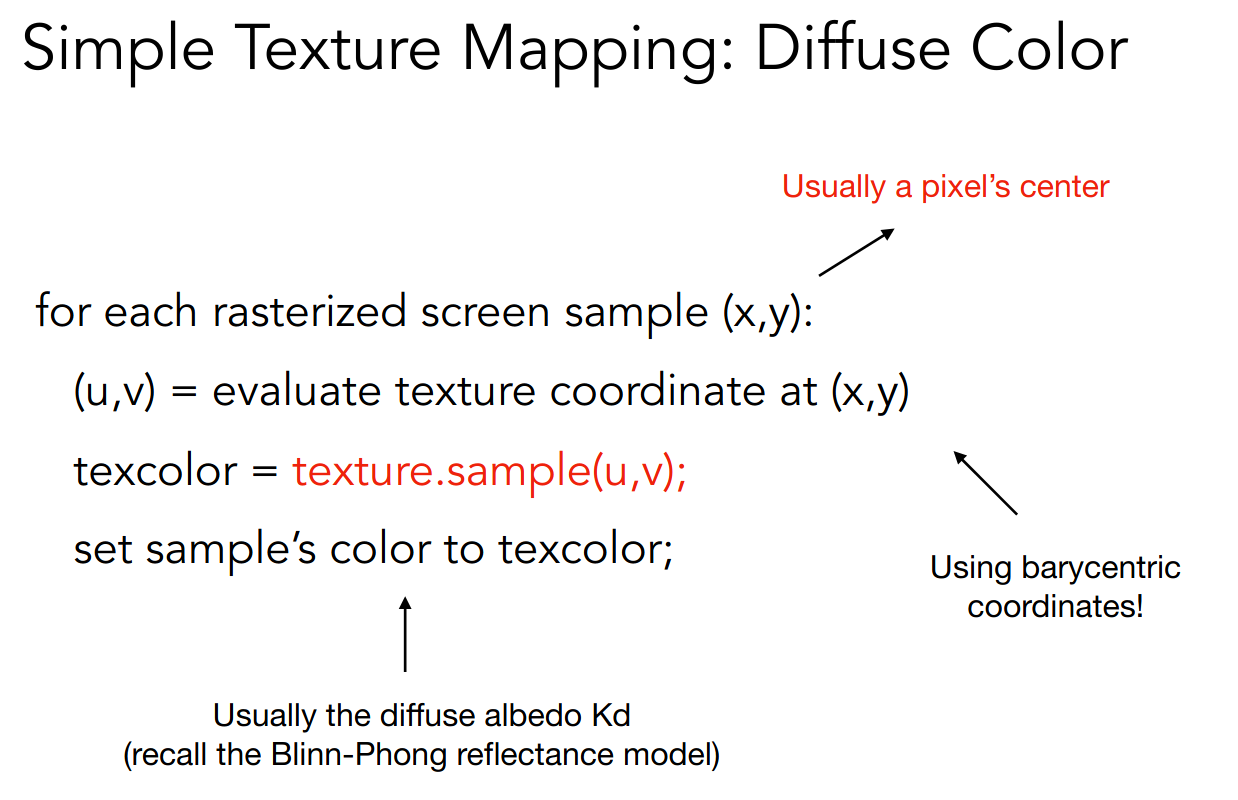
得到纹理空间的坐标后,还可能需要插值处理
感觉图中箭头指向的位置不太对
着色(插值、高级纹理映射)
Barycentric Coordinates
之前在许多地方都遇到了插值
- 深度测试
- 法向量
- 纹理
- ……
通过三角形的重心坐标实现插值,公式如下
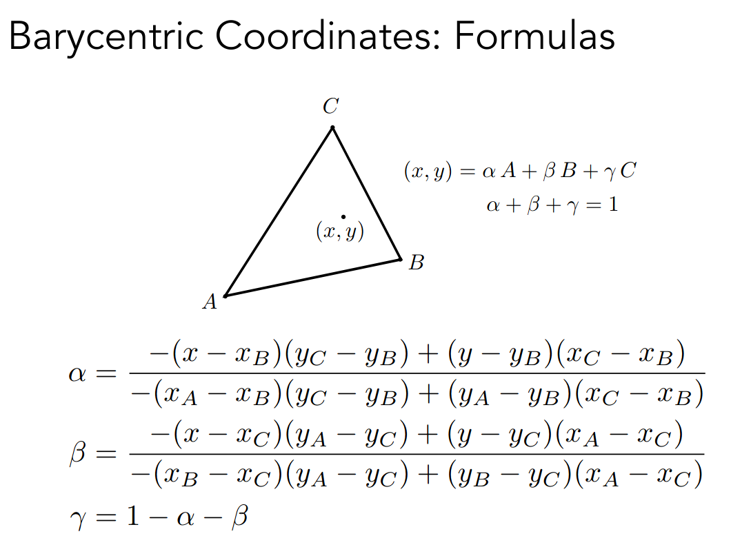
面积关系可以直观的理解
我们以插值颜色为例
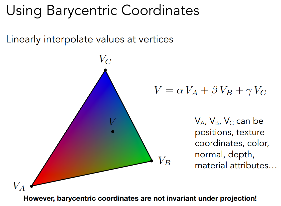
需要注意在投影变换下插值坐标可能发生变化
所以三维的属性在投影之前就应该进行插值
Texture antialiasing
What if the texture is too small?
纹理的分辨率太低
我们定义 pixel on a texture 为 texel
下面介绍双线性插值
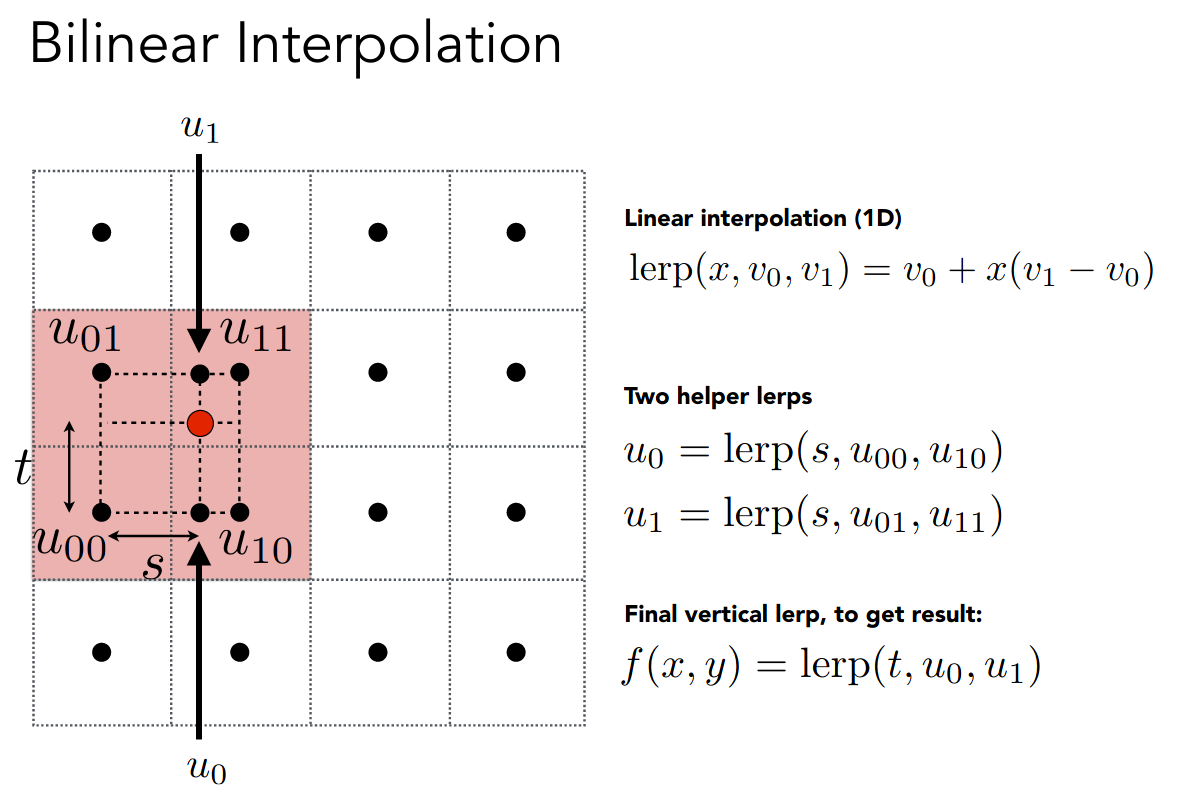
红色点是映射之后的坐标,而黑色点则是 texel
找最近的四个点,在两个方向线性插值即可
可以认为是正方形的重心坐标
当然还有效果更好的插值方法,如双三次插值 Bicubic Interpolation
What if the texture is too large?
通常是映射后所占据的纹理空间过大
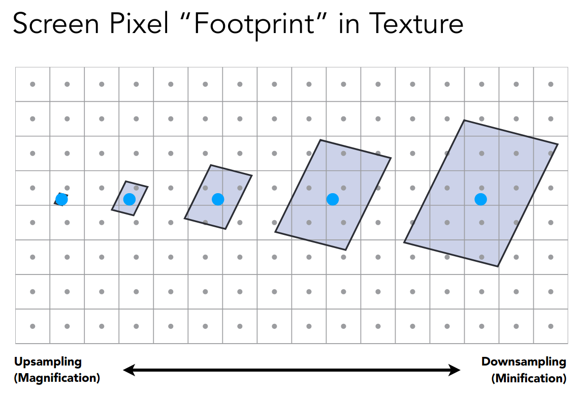
当然超采样是一种解决方案
我们考虑换一个思路,之前都是试图求纹理空间某个点对应的值
现在我们尝试求纹理空间某个范围对内应的统计量,如平均值或极值
这实际上就是二维的 range queries
有一个近似的解决方案为 Mipmap
Allowing (fast, approx., square) range queries
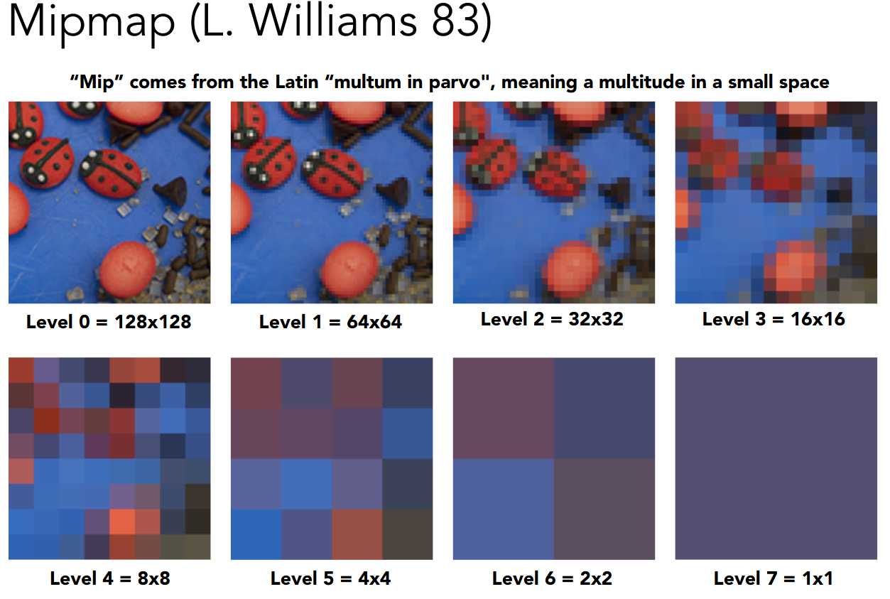
先对纹理空间进行预处理,所占用的额外空间不超过原占用空间的三分之一
然后通过某种方式得到查询范围的边长 L,并计算层级 D
接着在层级中进行双线性插值
最后在层级间进行线性插值,因为 D 可能不是整数
示意图如下,这也被称为三线性插值
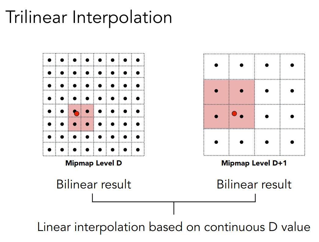
然而 Mipmap 对非正方形的处理误差会较大
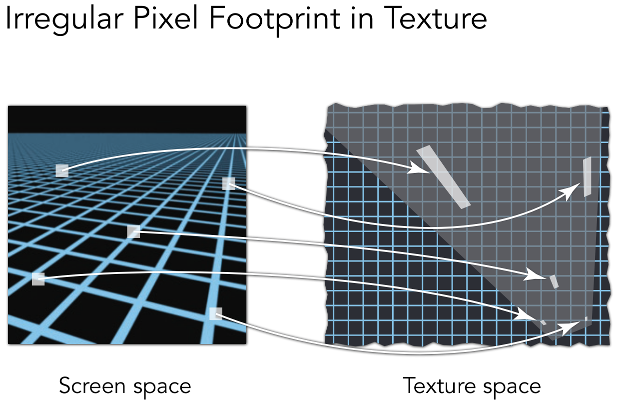
于是便有了各向异性过滤 Anisotropic Filtering,来处理矩阵的情形
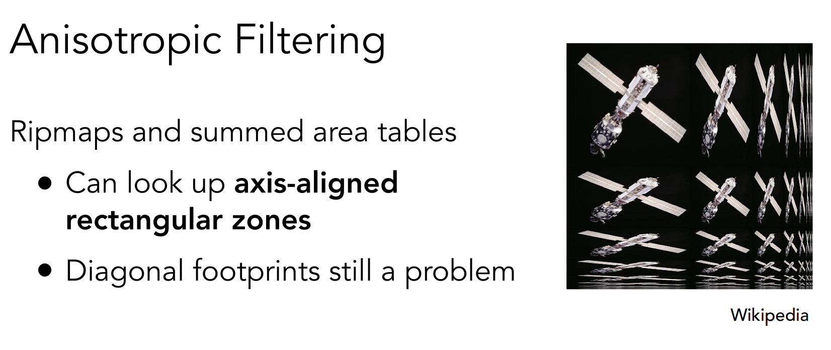
所占用的额外空间不超过原占用空间的三倍
然而各向异性过滤对于不规则的空间仍不易处理,可以参考 EWA filtering
PA3
run
./build/Rasterizer pa3-normal.png normalmv pa3-normal.png ~/Desktop/virtual-machine-repository/post/games101.assets/似乎不支持实时旋转
interface
需要使用的 eigen 方法
cwiseProduct对应元素相乘norm计算 L2 范数normalized单位化
note
首先需要修改一下 models 的路径
修改函数 rasterize_triangle
依次实现颜色、法向量、纹理颜色、纹理坐标的插值
        if (z_interpolated < depth_buf[get_index(i, j)]) {          depth_buf[get_index(i, j)] = z_interpolated;
          // TODO: Interpolate the attributes:          // auto interpolated_color          // auto interpolated_normal          // auto interpolated_texcoords          // auto interpolated_shadingcoords          auto interpolated_color = interpolate(alpha, beta, gamma, t.color[0],                                                t.color[1], t.color[2], 1);          auto interpolated_normal = interpolate(              alpha, beta, gamma, t.normal[0], t.normal[1], t.normal[2], 1);          auto interpolated_texcoords =              interpolate(alpha, beta, gamma, t.tex_coords[0], t.tex_coords[1],                          t.tex_coords[2], 1);          auto interpolated_shadingcoords =              interpolate(alpha, beta, gamma, view_pos[0], view_pos[1],                          view_pos[2], 1);
          fragment_shader_payload payload(              interpolated_color, interpolated_normal.normalized(),              interpolated_texcoords, texture ? &*texture : nullptr);          payload.view_pos = interpolated_shadingcoords;
          // Instead of passing the triangle's color directly to the frame          // buffer, pass the color to the shaders first to get the final color.          auto pixel_color = fragment_shader(payload);          frame_buf[get_index(i, j)] = pixel_color;        }
最终的颜色通过调用着色器函数 fragment_shader 得到
另外 insideTriangle 的参数类型有细微变化,Vector3f -> Vector4f
使用框架代码,将整型改为浮点型
修改函数 get_projection_matrix
Eigen::Matrix4f get_projection_matrix(float eye_fov, float aspect_ratio,                                      float zNear, float zFar) {  // TODO: Use the same projection matrix from the previous assignments  Eigen::Matrix4f projection;
  float yTop = zNear * std::tan(eye_fov / 360 * MY_PI);  float xRight = yTop * aspect_ratio;
  // clang-format off  Eigen::Matrix4f ortho_scale;  ortho_scale << 1 / xRight, 0, 0, 0,                 0, 1 / yTop, 0, 0,                 0, 0, 2 / (zFar - zNear), 0,                 0, 0, 0, 1;
  Eigen::Matrix4f ortho_trans;  ortho_trans << 1, 0, 0, 0,                 0, 1, 0, 0,                 0, 0, 1, (zNear + zFar) / 2,                 0, 0, 0, 1;
  Eigen::Matrix4f persp;  persp << zNear, 0, 0, 0,           0, zNear, 0, 0,           0, 0, zNear + zFar, -zNear * zFar,           0, 0, -1, 0; // attention -1
  projection = ortho_scale               * ortho_trans               * persp               * projection;  // clang-format on
  std::cout << projection << std::endl;
  return projection;}
之前的实现没有考虑到 ortho_trans
可以通过注释 clang-format 调整自动格式化的范围
修改函数 phong_fragment_shader,通过 Blinn-Phong reflectance model 计算 Fragment Color
Eigen::Vector3ftexture_fragment_shader(const fragment_shader_payload &payload) {  Eigen::Vector3f return_color = {0, 0, 0};  if (payload.texture) {    // TODO: Get the texture value at the texture coordinates of the current    // fragment    return_color = payload.texture->getColor(payload.tex_coords.x(),                                             payload.tex_coords.y());  }  Eigen::Vector3f texture_color;  texture_color << return_color.x(), return_color.y(), return_color.z();
  Eigen::Vector3f ka = Eigen::Vector3f(0.005, 0.005, 0.005);  Eigen::Vector3f kd = texture_color / 255.f;  Eigen::Vector3f ks = Eigen::Vector3f(0.7937, 0.7937, 0.7937);
  auto l1 = light{{20, 20, 20}, {500, 500, 500}};  auto l2 = light{{-20, 20, 0}, {500, 500, 500}};
  std::vector<light> lights = {l1, l2};  Eigen::Vector3f amb_light_intensity{10, 10, 10};  Eigen::Vector3f eye_pos{0, 0, 10};
  float p = 150;
  Eigen::Vector3f color = texture_color;  Eigen::Vector3f point = payload.view_pos;  Eigen::Vector3f normal = payload.normal;  Eigen::Vector3f view_vec = eye_pos - point;  Eigen::Vector3f result_color = {0, 0, 0};
  for (auto &light : lights) {    // TODO: For each light source in the code, calculate what the *ambient*,    // *diffuse*, and *specular* components are. Then, accumulate that result on    // the *result_color* object.    Eigen::Vector3f light_vec = light.position - point;    Eigen::Vector3f half_vec = view_vec + light_vec;    float n_dot_l = normal.dot(light_vec.normalized());    float n_dot_h = normal.dot(half_vec.normalized());    float r_square = light_vec.dot(light_vec);    result_color += ka.cwiseProduct(amb_light_intensity);    result_color +=        kd.cwiseProduct(light.intensity) / r_square * std::max(0.f, n_dot_l);    result_color += ks.cwiseProduct(light.intensity) / r_square *                    std::pow(std::max(0.f, n_dot_h), p);  }
  return result_color * 255.f;}
直接看有纹理的版本
修改函数 bump_fragment_shader,实现 Bump mapping
Eigen::Vector3f bump_fragment_shader(const fragment_shader_payload &payload) {  assert(payload.texture);
  Eigen::Vector3f ka = Eigen::Vector3f(0.005, 0.005, 0.005);  Eigen::Vector3f kd = payload.color;  Eigen::Vector3f ks = Eigen::Vector3f(0.7937, 0.7937, 0.7937);
  auto l1 = light{{20, 20, 20}, {500, 500, 500}};  auto l2 = light{{-20, 20, 0}, {500, 500, 500}};
  std::vector<light> lights = {l1, l2};  Eigen::Vector3f amb_light_intensity{10, 10, 10};  Eigen::Vector3f eye_pos{0, 0, 10};
  float p = 150;
  Eigen::Vector3f color = payload.color;  Eigen::Vector3f point = payload.view_pos;  Eigen::Vector3f normal = payload.normal;
  float kh = 0.2, kn = 0.1;
  // TODO: Implement bump mapping here  // Let n = normal = (x, y, z)  // Vector t = (x*y/sqrt(x*x+z*z),sqrt(x*x+z*z),z*y/sqrt(x*x+z*z))  // Vector b = n cross product t  // Matrix TBN = [t b n]  // dU = kh * kn * (h(u+1/w,v)-h(u,v))  // dV = kh * kn * (h(u,v+1/h)-h(u,v))  // Vector ln = (-dU, -dV, 1)  // Normal n = normalize(TBN * ln)  Eigen::Vector3f t{      normal.x() * normal.y() /          std::sqrt(normal.x() * normal.x() + normal.z() * normal.z()),      std::sqrt(normal.x() * normal.x() + normal.z() * normal.z()),      normal.z() * normal.y() /          std::sqrt(normal.x() * normal.x() + normal.z() * normal.z())};  Eigen::Vector3f b{normal.cross(t)};  Eigen::Matrix3f TBN;  // clang-format off  TBN << t.x(), b.x(), normal.x(),         t.y(), b.y(), normal.y(),         t.z(), b.z(), normal.z();  // clang-format on  float u = payload.tex_coords.x();  float v = payload.tex_coords.y();  int w = payload.texture->width;  int h = payload.texture->height;  float dU = kh * kn *             (payload.texture->getColor(u + 1.f / w, v).norm() -              payload.texture->getColor(u, v).norm());  float dV = kh * kn *             (payload.texture->getColor(u, v + 1.f / h).norm() -              payload.texture->getColor(u, v).norm());  Eigen::Vector3f ln{-dU, -dV, 1.f};  normal = (TBN * ln).normalized();
  Eigen::Vector3f result_color = {0, 0, 0};  result_color = normal;
  return result_color * 255.f;}
这是后面的内容,属实有点超纲
注意 h(u,v) = texture_color(u,v).norm
其中 u,v 是 tex_coords
w,h 是 texture 的宽度与高度
displacement_fragment_shader 相当于多了 Blinn-Phong reflectance model 的部分
pic
感觉视角和 Bump mapping 实现的有点问题
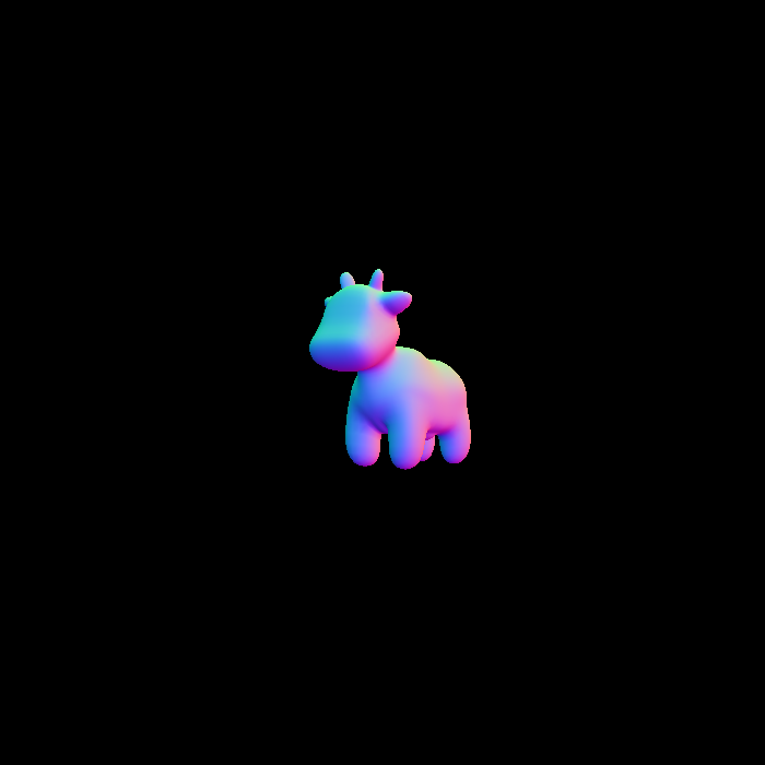
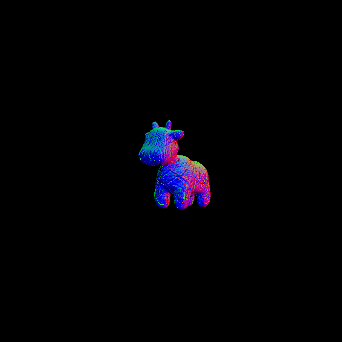
pa3-normal
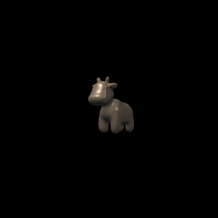
pa3-phong
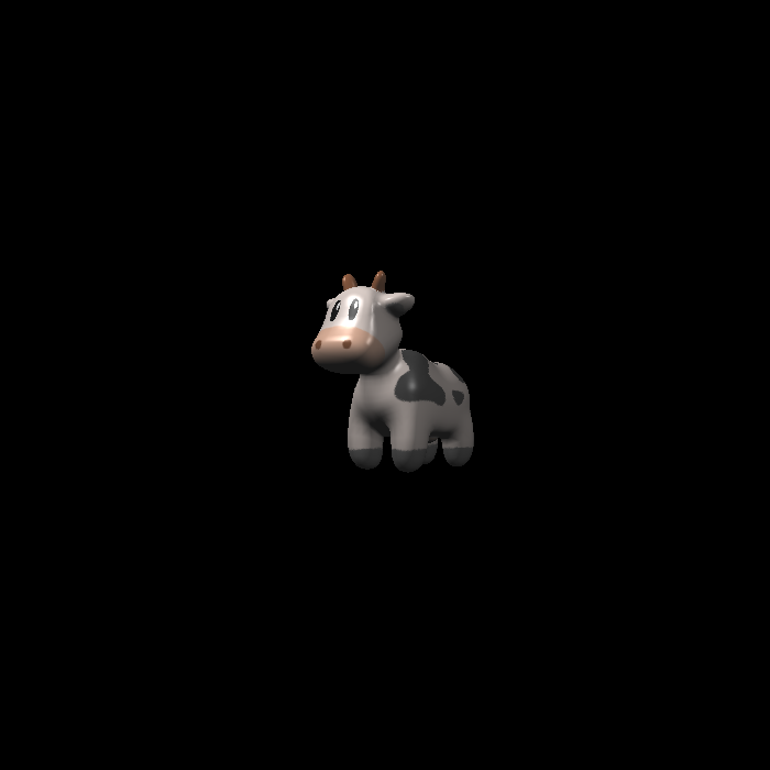
pa3-texture
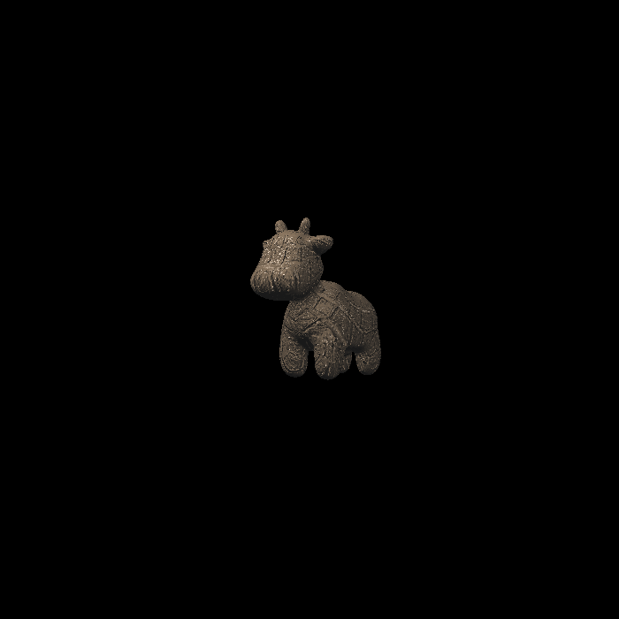
pa3-bump
pa3-displacement
todo
- debug
- 更多的 models
- 双线性纹理插值
几何(基本表示方法)
Applications of textures
着色最后的内容
一些纹理的应用
In modern GPUs, texture = memory + range query (filtering)
General method to bring data to fragment calculations
Environment Map
环境光贴图可以让模型反射出周围环境的样子
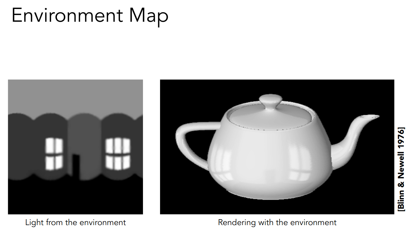
- Spherical Map
- Cube Map
Bump Mapping / Normal mapping
使用纹理空间表示 height 或 normal
以二维的 Bump Mapping 为例,扰动法线
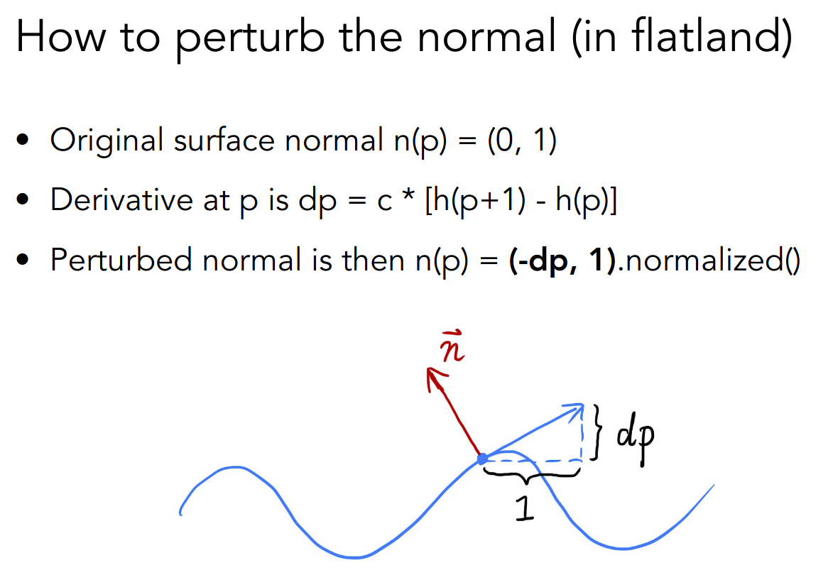
Displacement mapping
已经不太懂了
https://zhuanlan.zhihu.com/p/340786255
Ambient occlusion texture map
预先计算环境光遮蔽,并反映在纹理上
shadow
3D Textures
Introduction to geometry
Implicit Representations
Inside/Outside Tests Easy
- Algebraic Surfaces
解析式
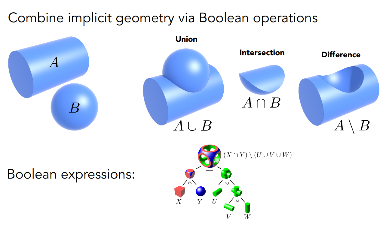
- Constructive Solid Geometry
使用布尔运算组合
- Distance Functions
记录到物体的最短距离
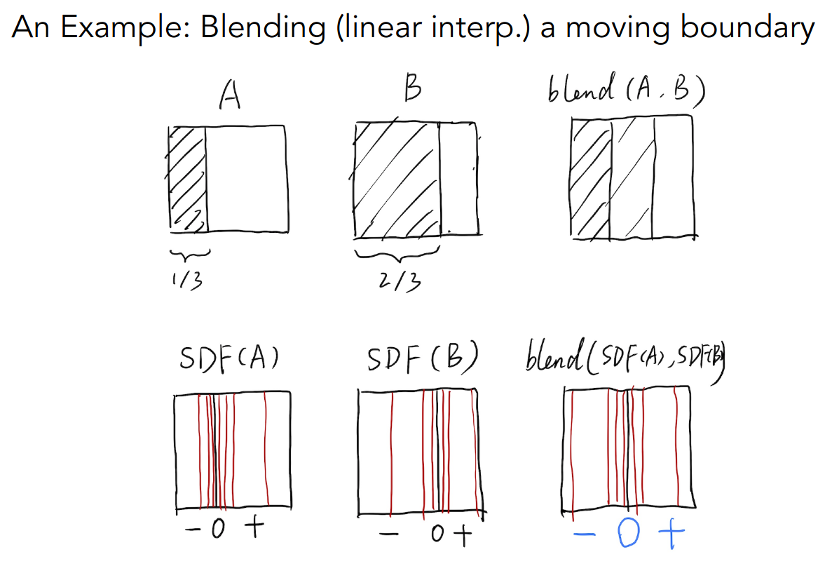
例如直接线性插值,中间部分就是灰色
使用有向距离函数变换后再 blend
中间部分的距离就是零,变换回来正好左边黑右边白
- Level Set Methods
类似等高线
- Fractals
分形结构
Explicit Representations
Sampling Is Easy
- All points are given directly or via parameter mapping
参数方程
如
几何(曲线与曲面)
Explicit Representations
- Point Cloud
顾名思义,一堆密集的点形成几何图形
- Polygon Mesh
存储顶点和多边形
- The Wavefront Object File
(.obj)Format
PA3 的 models 文件夹里有这种类型的文件
https://en.wikipedia.org/wiki/Wavefront_.obj_file
Curves
主要讲贝塞尔曲线 Bézier Curves
de Casteljau Algorithm
直接从代数的角度计算
以三次贝塞尔曲线为例,有四个控制点,一个参数
所以贝塞尔曲线是 Explicit Representations
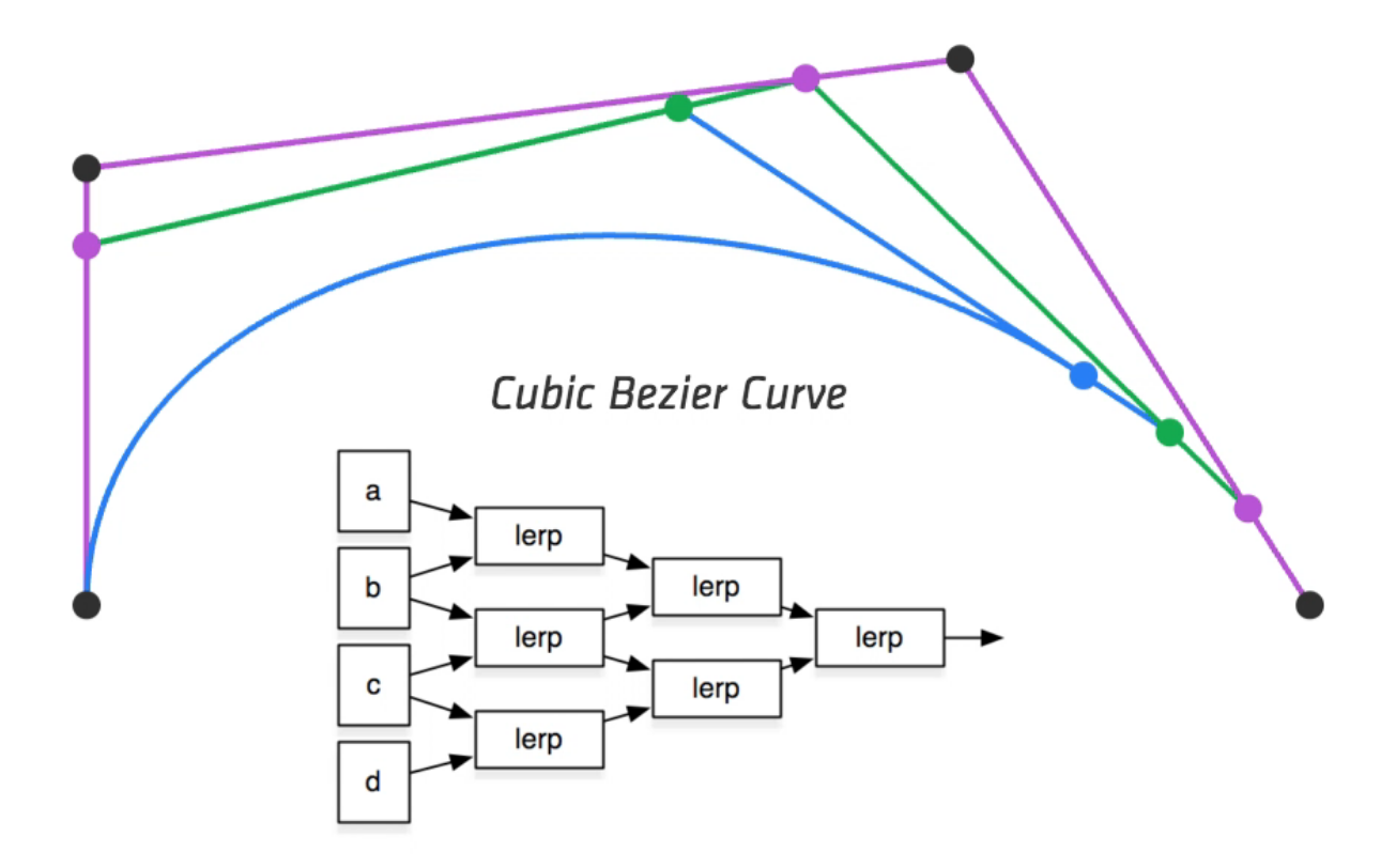
控制点之间做线性插值,得到新的控制点
然后递归进行,最终得到对应参数的点
Algebraic Formula
以二次贝塞尔曲线为例
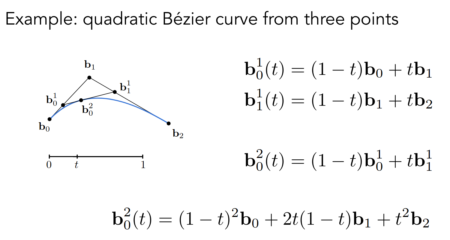
观察形式类似于二项展开
不难推出,对于 次贝塞尔曲线,有
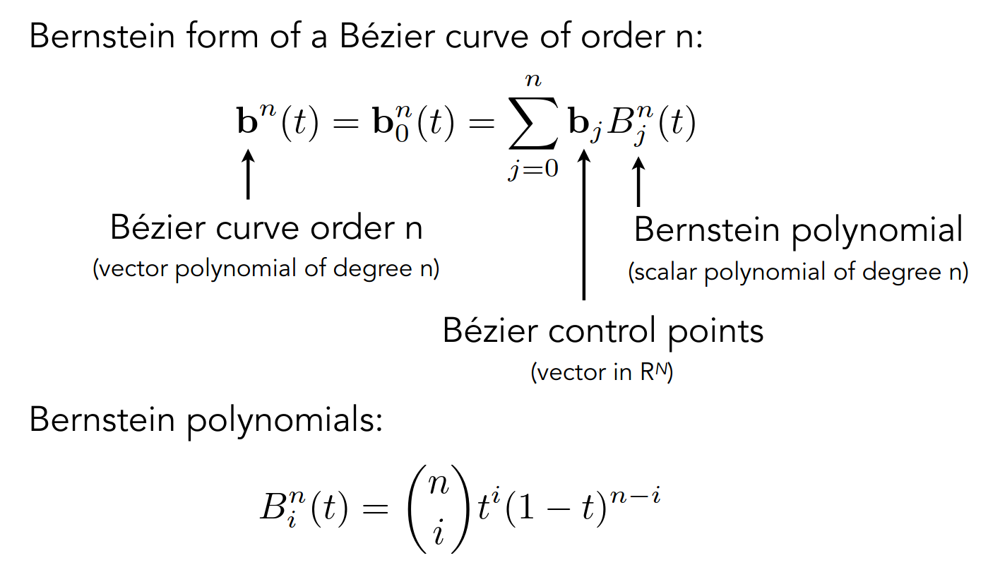
Properties of Bézier Curves
- 起点和终点与两端的控制点重合
- 可以计算出曲线两端的切线方向和大小
以三次贝塞尔曲线为例
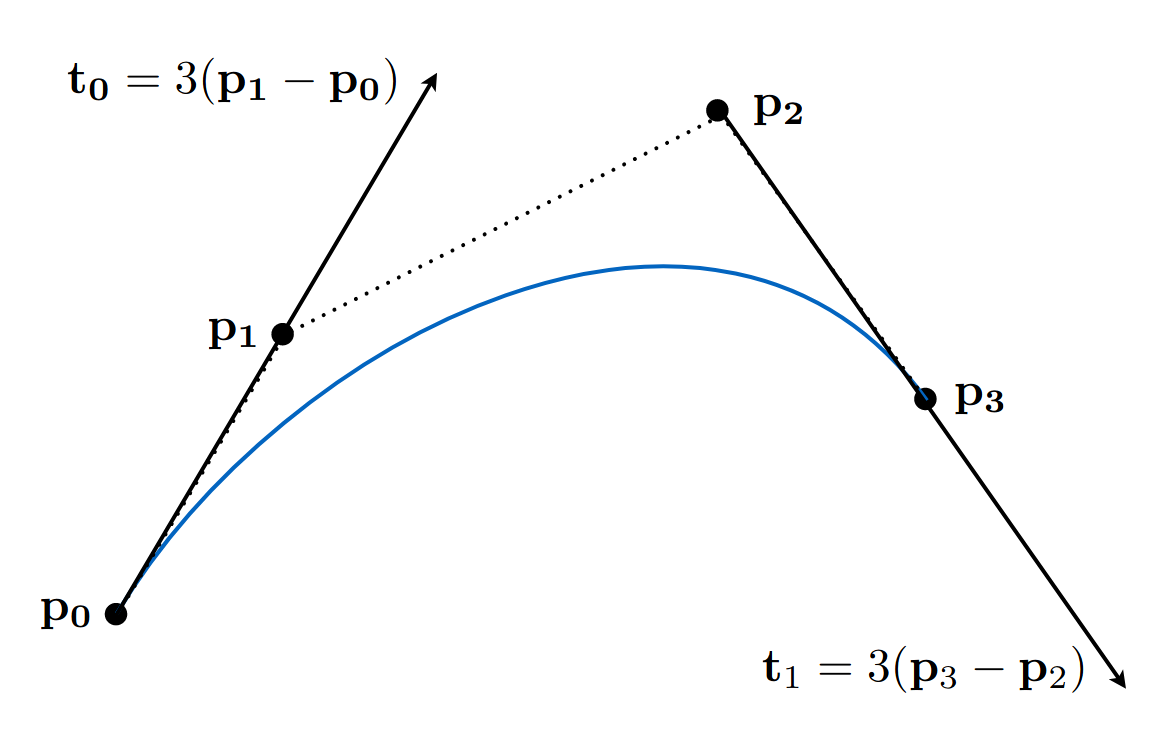
求导即可
- 仿射变换不变性
- 曲线在控制点构成多边形的闭包内
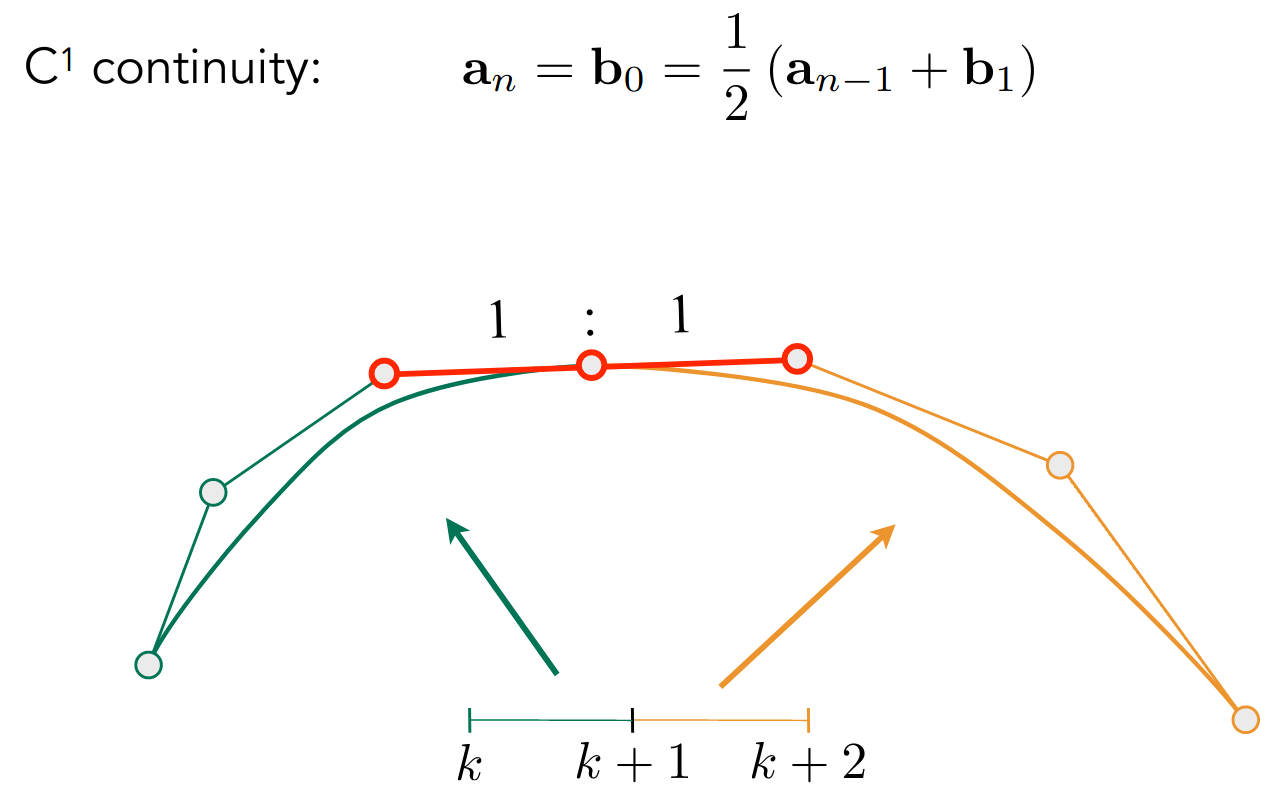
Piecewise Bézier Curves
分段贝塞尔曲线
通常使用三次贝塞尔曲线
https://math.hws.edu/eck/cs424/notes2013/canvas/bezier.html
下面讨论连续性
- 不中断可以保证 连续
- 而切线方向和大小相同可以保证 连续
Other types of splines
Bézier Curves 的超集
- B-splines
- NURBS
- ……
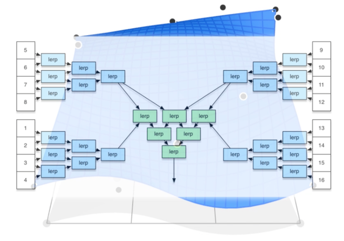
Surfaces
Bezier Surfaces
多引入一个参数
计算思路大致相同,只不过多一个维度
Mesh Operations
处理曲面的多边形
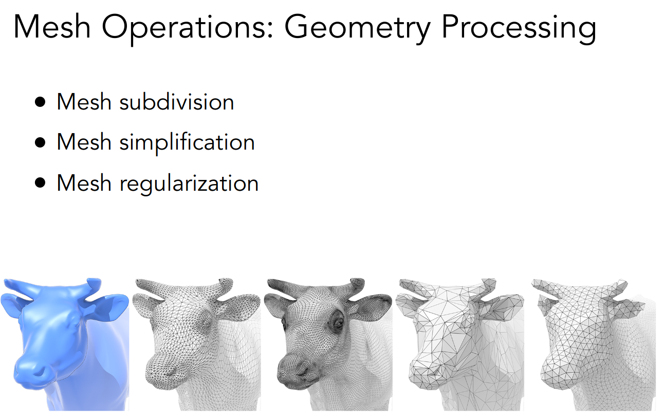
- 细分 - 第三幅图
- 简化 - 第四幅图
- 规范化 - 第五幅图
更多内容在下一节课
PA4
note
相当水
cv::Point2f recursive_bezier(const std::vector<cv::Point2f> &control_points,                             float t) {  // TODO: Implement de Casteljau's algorithm  if (control_points.size() == 2) {    return (1 - t) * control_points[0] + t * control_points[1];  }
  std::vector<cv::Point2f> new_control_points;
  for (size_t i = 0; i < control_points.size() - 1; ++i) {    new_control_points.emplace_back((1 - t) * control_points[i] +                                    t * control_points[i + 1]);  }
  return recursive_bezier(new_control_points, t);}
void bezier(const std::vector<cv::Point2f> &control_points, cv::Mat &window) {  // TODO: Iterate through all t = 0 to t = 1 with small steps, and call de  // Casteljau's recursive Bezier algorithm.
  assert(control_points.size() == count);
  for (double t = 0.0; t <= 1.0; t += step) {    auto point = recursive_bezier(control_points, t);
    window.at<cv::Vec3b>(point.y, point.x)[1] = 255; // green  }}
另外还实现了通用的 naive_bezier
使用了 C++17 中的 beta 函数计算二项展开系数
double binom(int n, int k) {  return 1 / ((n + 1) * std::beta(n - k + 1, k + 1));}
void naive_bezier(const std::vector<cv::Point2f> &points, cv::Mat &window) {  assert(points.size() == count);
  for (double t = 0.0; t <= 1.0; t += step) {    cv::Point2f point{};    for (size_t i = 0; i < points.size(); ++i) {      point += binom(count - 1, i) * std::pow(1 - t, count - 1 - i) *               std::pow(t, i) * points[i];    }
    window.at<cv::Vec3b>(point.y, point.x)[2] = 255; // blue  }}
需要修改 mouse_handler 和 main 中的控制点数量以实现任意阶的贝塞尔曲线
还有光栅化的时候坐标似乎不是整数
window.at<cv::Vec3b>(point.y, point.x)[1] = 255;为什么 x 和 y 颠倒了
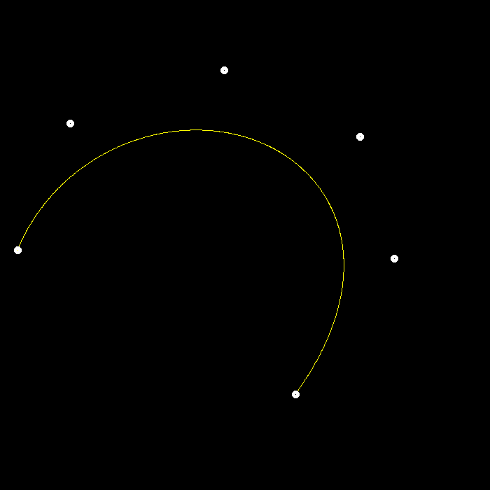
pic
五阶贝塞尔曲线
同时使用 bezier 和 naive_bezier 绘制
todo
- 反走样
几何(网格处理)、阴影图
Mesh Subdivision
Loop Subdivision
Loop 是人名
只对三角形面有效
分两步
- Split each triangle into four
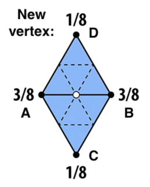
- Assign new vertex positions according to weights
- New / old vertices updated differently
对于新生成的顶点,根据下图分配权重
对于原本的顶点
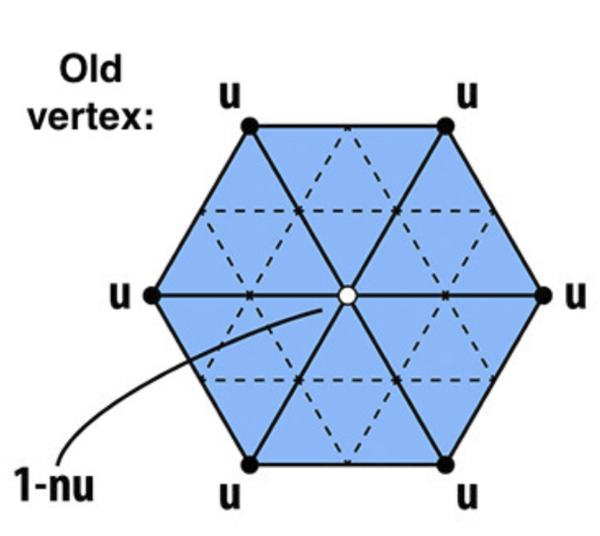
需要得到该顶点的度 ,然后根据 设置权重
这样可以保证当 较小时,顶点自身的权重较大,而当 较大时,顶点自身的权重较小
Catmull-Clark Subdivision
可用于任意多边形面
同样分两步走,首先看如何 split
第一步,在每个面的中心添加一个点,该点与这个面各边的中点相连
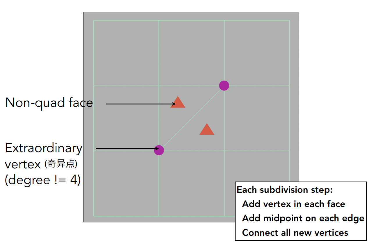
第一步过后,奇异点的数量会增加某个值,该值等于原图中非四边形面的数量
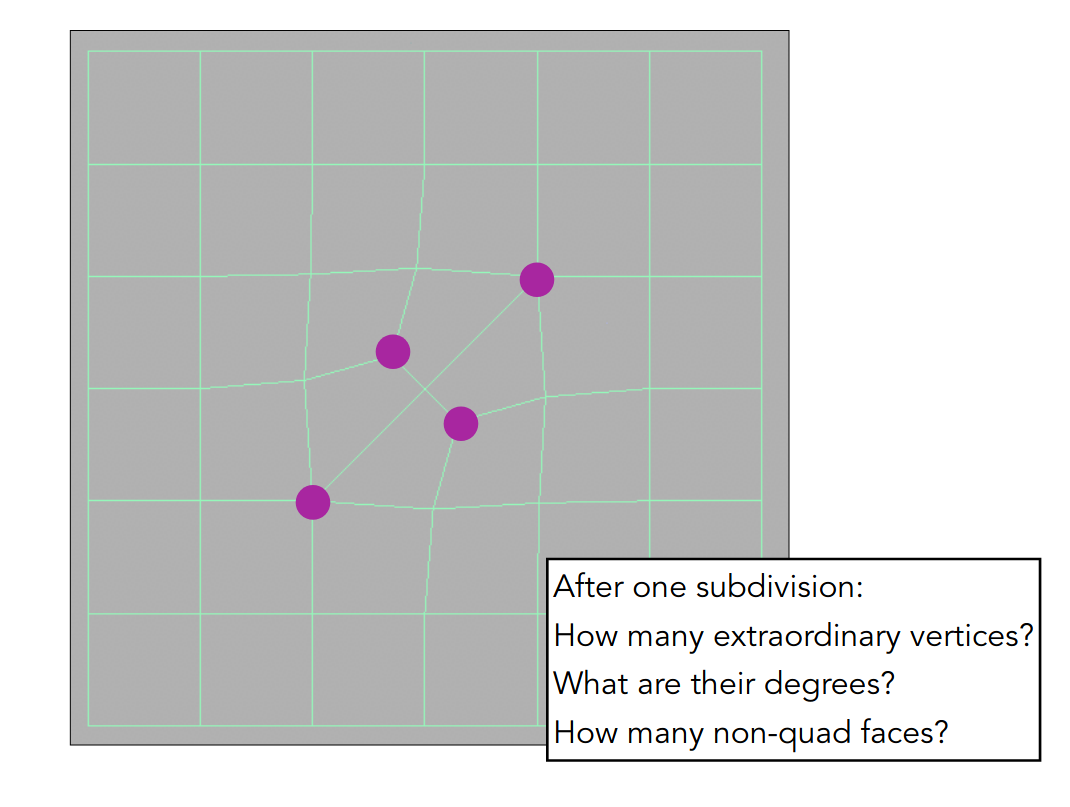
之后重复上述操作,可以证明奇异点的数量不会改变
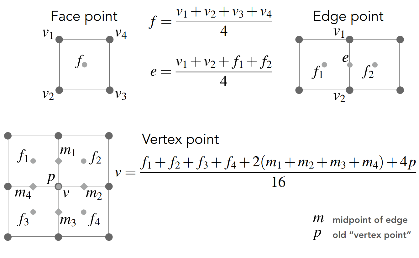
下面考虑权重问题,直接给出公式
Mesh Simplification
Suppose we simplify a mesh using edge collapsing
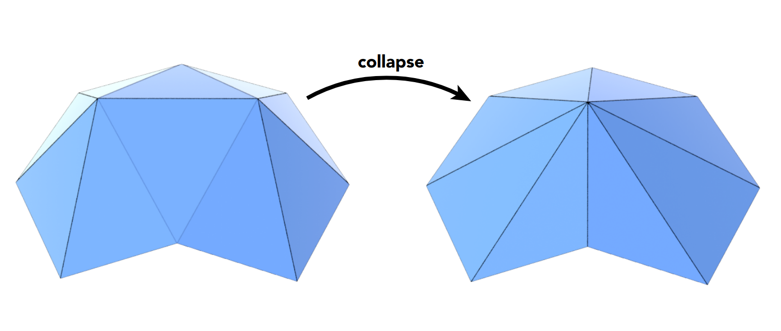
相当于将一条边的两个端点变为一个点
为了计算变换的误差,需要引入二次误差度量
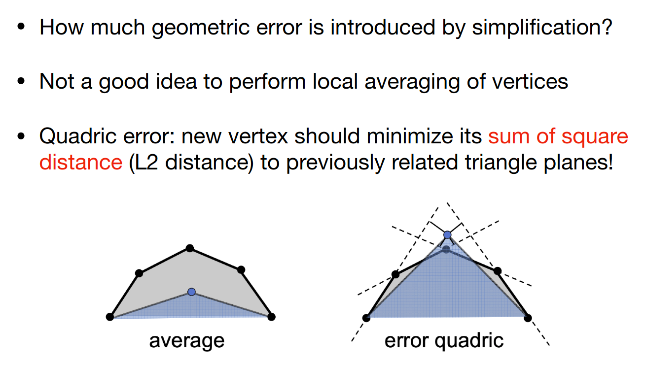
也就是该点与原相邻面距离的平方和
对于曲面中的每一条边,都可以计算出对应二次误差度量的最小值
以从小到大的顺序进行 edge collapsing 即可
注意每进行一步 edge collapsing,可能需要重新计算某些边对应二次误差度量的最小值
本质上是贪心算法,不保证能找到最优解,不过实际中效果还不错
Shadow Mapping
光线追踪的导论
之前提过,光栅化的着色不考虑 shadow
现在考虑点光源产生的硬阴影
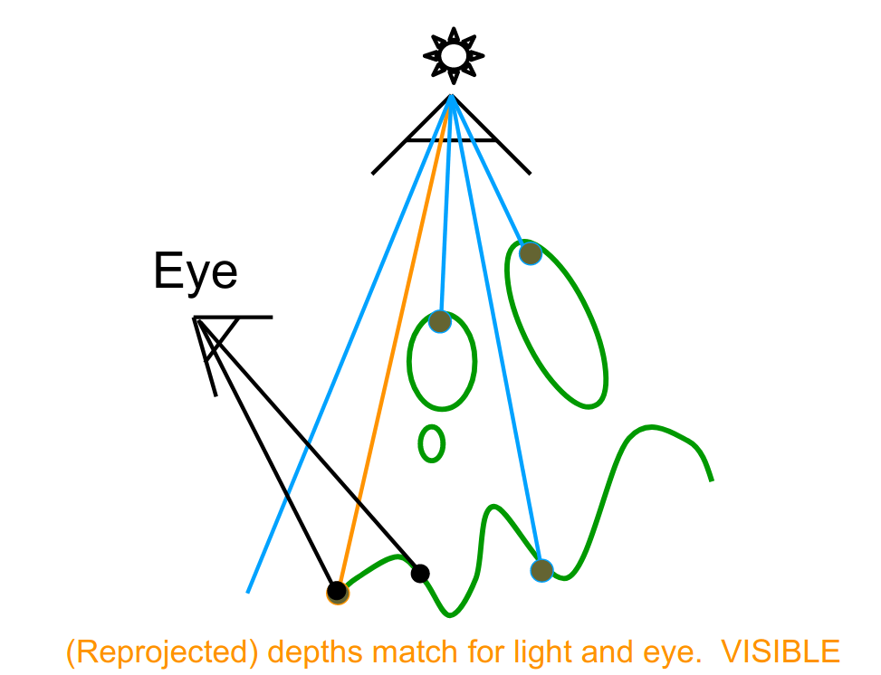
关键思想是 the points NOT in shadow must be seen both by the light and by the camera
所以着色要分为两轮
- 从点光源的方向看场景,进行深度测试,得到 Shadow Mapping
- 从相机的方向看场景,对于每一个点,反向应用 Shadow Mapping 得到点光源的方向的深度值,并进行比较
可见的情形
不可见的情形
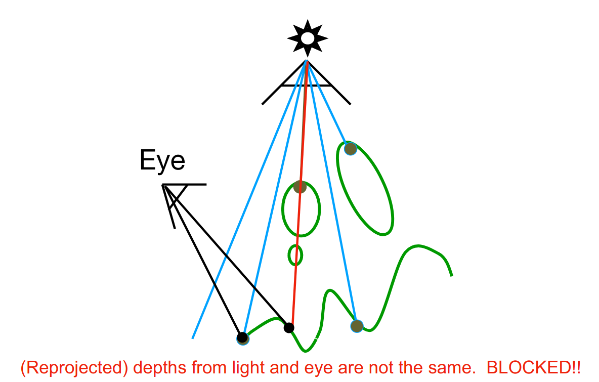
这种方法得到的 shadow 可能会出现走样,取决于 Shadow Mapping 的采样率
下面区分一下硬阴影和软阴影
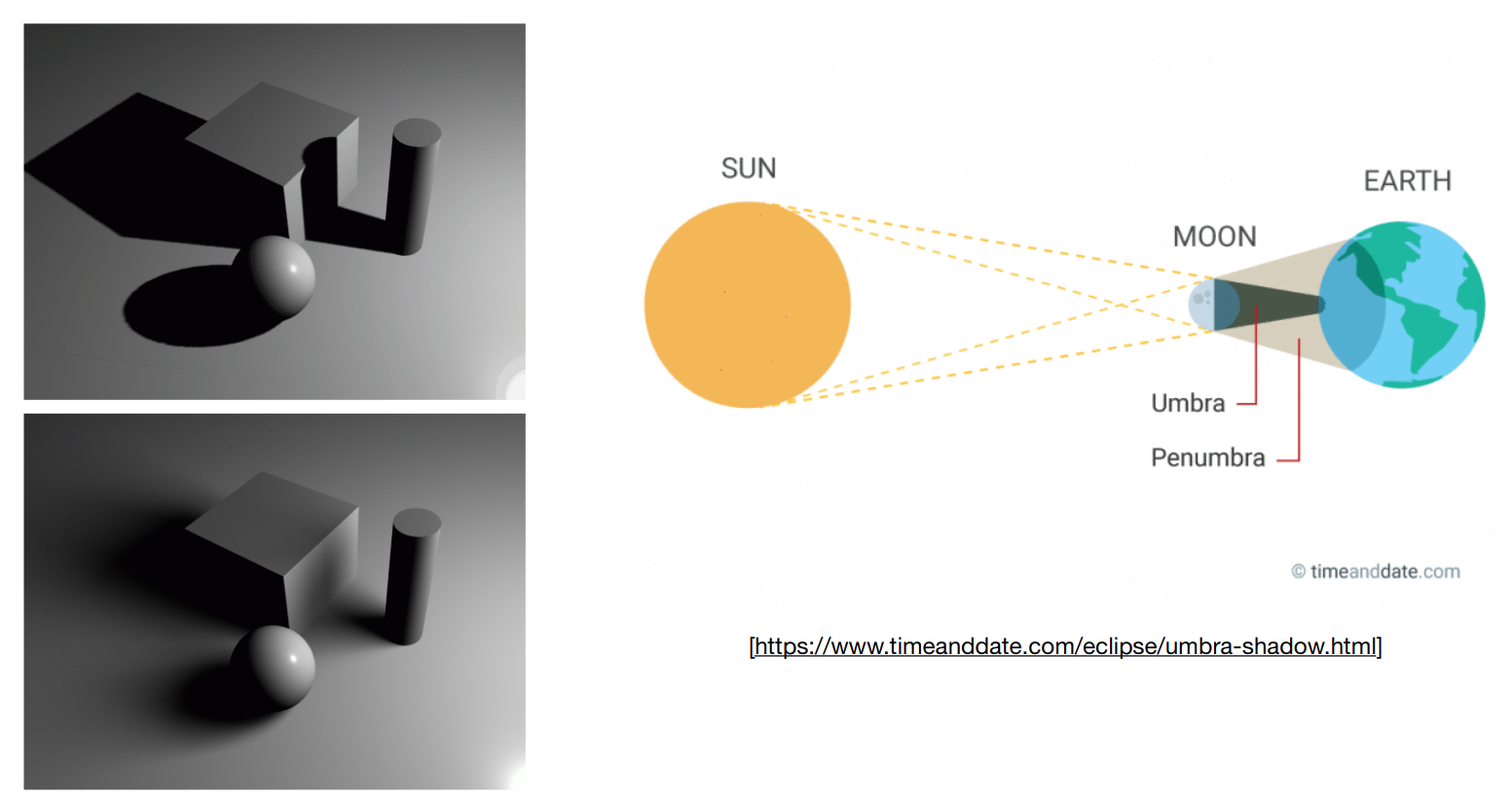
软阴影中阴影的渐变效果,本质上是因为光源有一定的大小,而非点光源
光线追踪(基本原理)
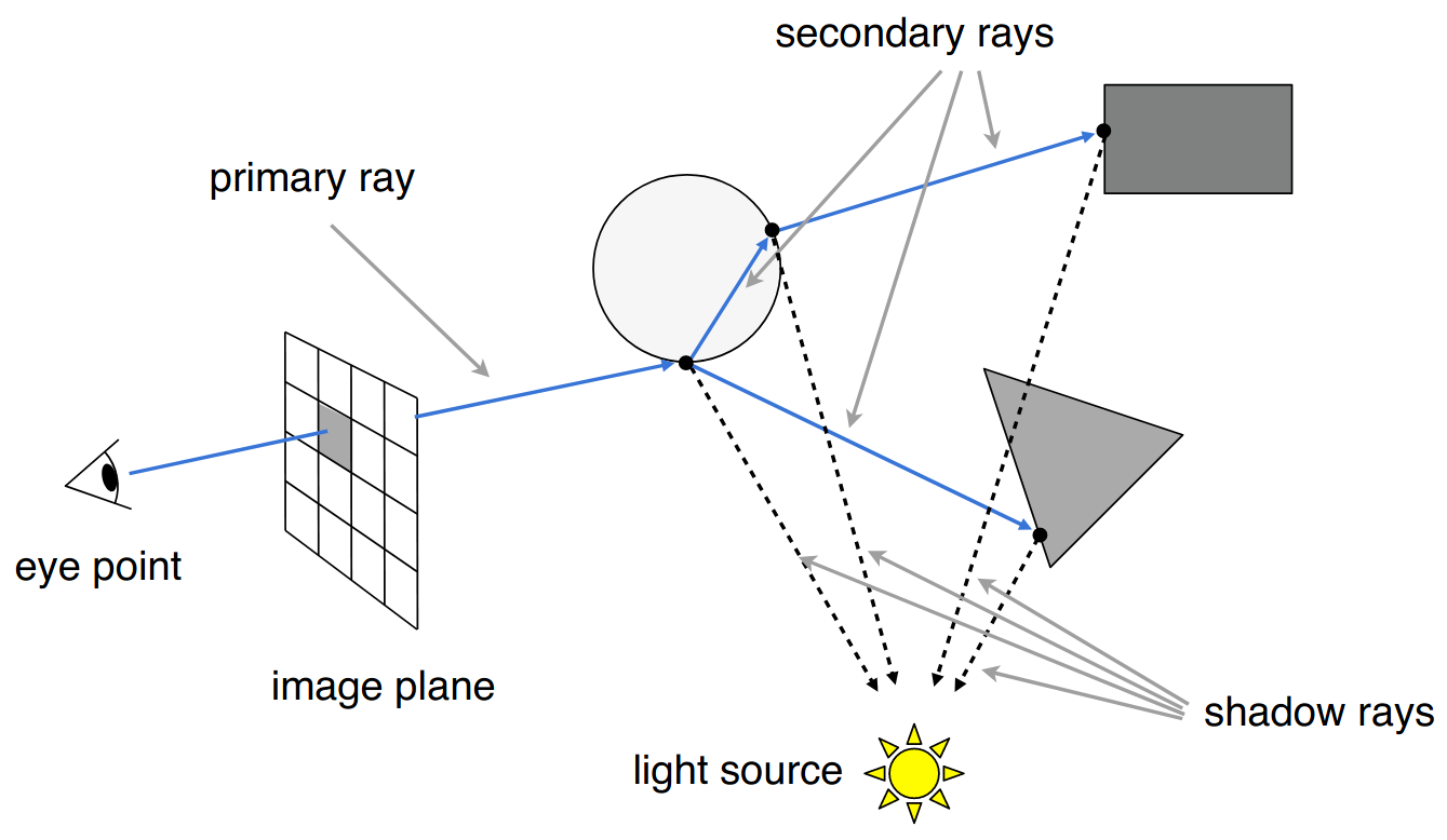
Basic Ray-Tracing Algorithm
对光线的假设
- 光线沿直线传播
- 光线之间没有干扰
- 光路可逆
只要考虑到光线的反射和折射,并使用 Blinn-Phong reflectance model 叠加着色,就是最基本的光线追踪算法
Recursive (Whitted-Style) Ray Tracing
下面考虑一些技术细节
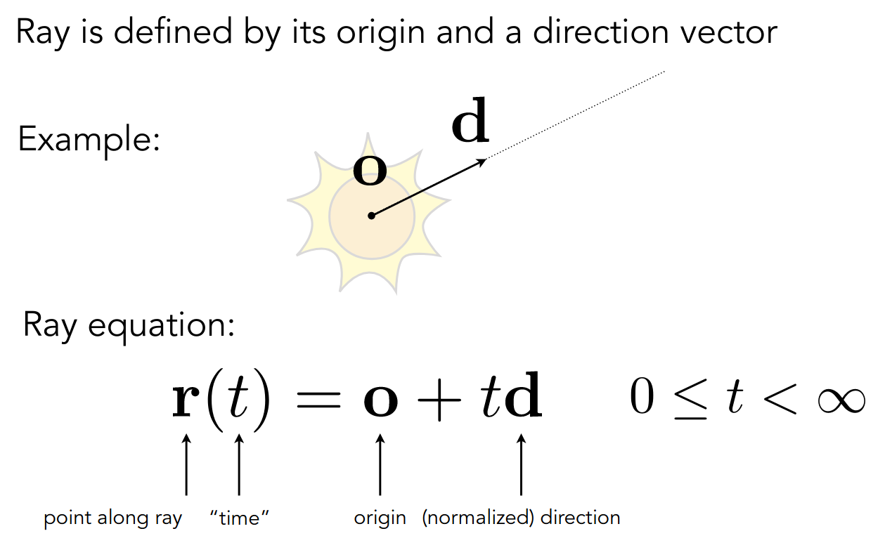
Ray-Surface Intersection
需要求出光线和几何表面的交点
首先需要为光线建模,实际上就是一条射线
Implicit Surfaces
以 Algebraic Surfaces 为例
只需要联立下面两式
求出正实数解 即可
Explicit Surfaces
以 Polygon Mesh 为例
首先考虑一个简单的算法,对光线和几何表面的每个三角形求交点
光线和三角形求交,实际上可以分解为
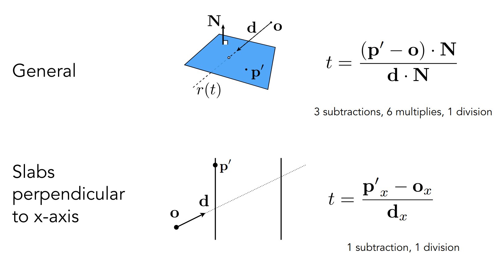
- 光线和平面求交
- 交点是否在三角形内(外积)
所以只要考虑光线和平面求交,使用点法式表示平面方程
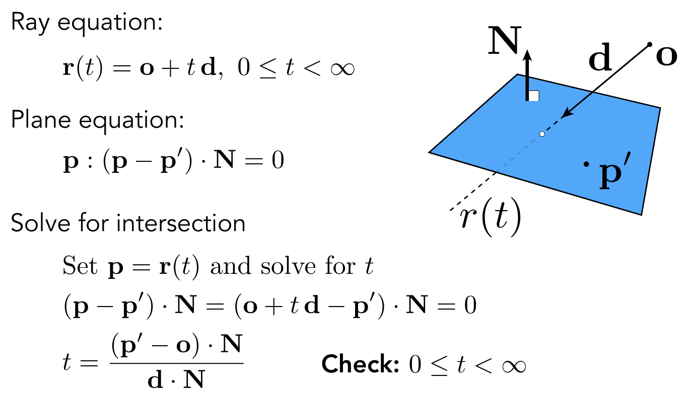
联立即可解出
一个优化是直接考虑光线和三角形求交
即 Möller Trumbore Algorithm
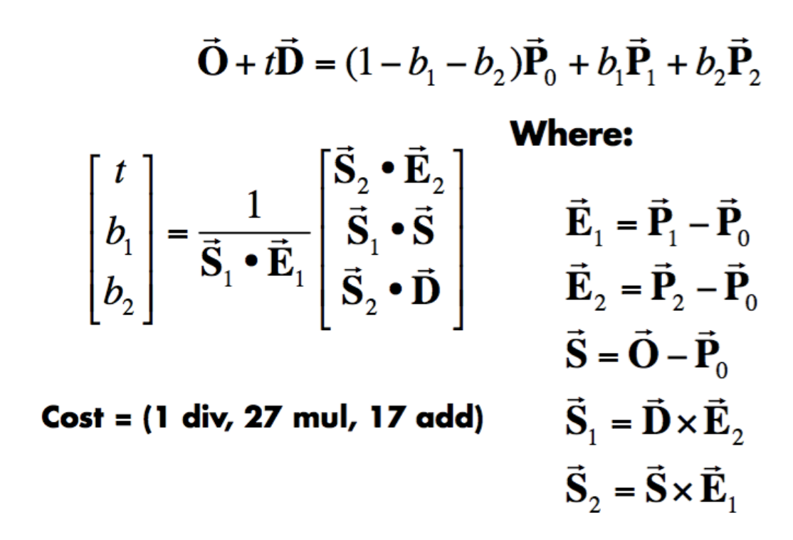
使用重心坐标表示交点
向量的维度为
有三个未知量
也就是一个线性方程组
Accelerating Ray-Surface Intersection
当场景中三角形数量较多时,或者像素点数量较多时
对光线和几何表面的每个三角形求交点,实际上至少需要计算这么多次
pixels x traingle x bounces我们使用 Bounding Volumes 加速
Bounding Volumes
当光线和 Bounding Volumes 都不相交时,肯定不会与 Surface 相交
为了计算方便,我们使用 Axis-Aligned Bounding Box (AABB)
核心算法如下,我们视 Bounding Volumes 为三对平面相交的部分
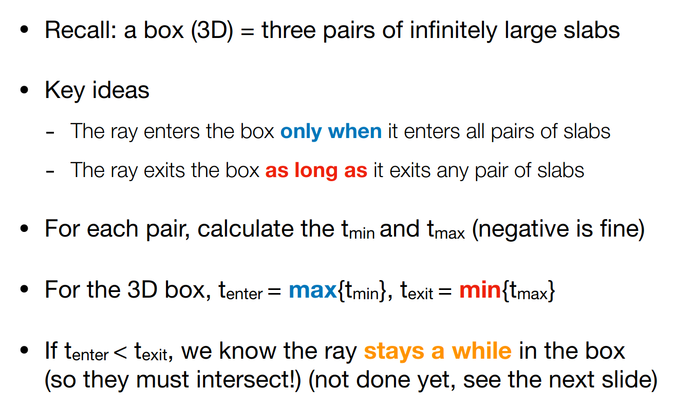
求出光线进入三对平面的 和光线离开三对平面的
即可得出光线在 Bounding Volumes 内部的时间段
满足如下两个条件
即可判定光线和 Bounding Volumes 相交
也无所谓,代表光线源点在 Bounding Volumes 内部
而关于计算 ,由于平面和坐标轴对齐,所以只考虑一个分量即可
PA5
竟然没有使用任何第三方库……
Render
原理如下
可能是因为相机朝向 -z 轴,所以计算 y 轴分量时需要取负
另外别忘了加上 0.5
  for (int j = 0; j < scene.height; ++j) {    for (int i = 0; i < scene.width; ++i) {      // generate primary ray direction      float x;      float y;      // TODO: Find the x and y positions of the current pixel to get the      // direction vector that passes through it. Also, don't forget to multiply      // both of them with the variable *scale*, and x (horizontal) variable      // with the *imageAspectRatio*      x = (((i + 0.5) / (float)scene.width) * 2 - 1) * scale * imageAspectRatio;      y = (1 - ((j + 0.5) / (float)scene.height * 2)) * scale;      // y = (((j + 0.5) / (float)scene.height) * 2 - 1) * scale;
      Vector3f dir = normalize(          Vector3f(x, y, -1)); // Don't forget to normalize this direction!      framebuffer[m++] = castRay(eye_pos, dir, scene, 0);    }    UpdateProgress(j / (float)scene.height);  }
本质上是映射
rayTriangleIntersect
是三角形的三个顶点
是光线的起点
是光线单位化的方向向量
是需要使用 Möller Trumbore Algorithm 来更新的参数
bool rayTriangleIntersect(const Vector3f &v0, const Vector3f &v1,                          const Vector3f &v2, const Vector3f &orig,                          const Vector3f &dir, float &tnear, float &u,                          float &v) {  // TODO: Implement this function that tests whether the triangle  // that's specified bt v0, v1 and v2 intersects with the ray (whose  // origin is *orig* and direction is *dir*)  // Also don't forget to update tnear, u and v.  Vector3f e1 = v1 - v0;  Vector3f e2 = v2 - v0;  Vector3f s = orig - v0;  Vector3f s1 = crossProduct(dir, e2);  Vector3f s2 = crossProduct(s, e1);
  float denominator = dotProduct(s1, e1);  float _tnear = dotProduct(s2, e2) / denominator;  float _u = dotProduct(s1, s) / denominator;  float _v = dotProduct(s2, dir) / denominator;  if (_tnear >= 0 and 0 <= _u and _u <= 1 and 0 <= _v and _v <= 1 and      _u + _v <= 1) {    tnear = _tnear;    u = _u;    v = _v;    return true;  }
  return false;}
直接抄公式即可
注意限制条件
pic
使用 imagemagick 转换 ppm 为 png
$ convert pa5.ppm pa5.png光线追踪(加速结构)
上节课讲了如何计算光线和 Bounding Volumes 求交
这节课介绍如何利用 Bounding Volumes 加速光线和几何表面求交
以二维为例
Uniform Spatial Partitions (Grids)
首先需要将场景进行划分,进行预处理
考虑均匀划分
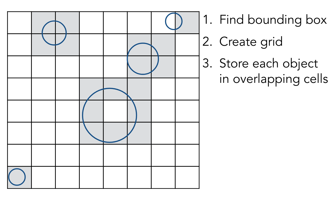
然后让光线与 grid 求交,若相交,且内部有物体,再去和物体求交
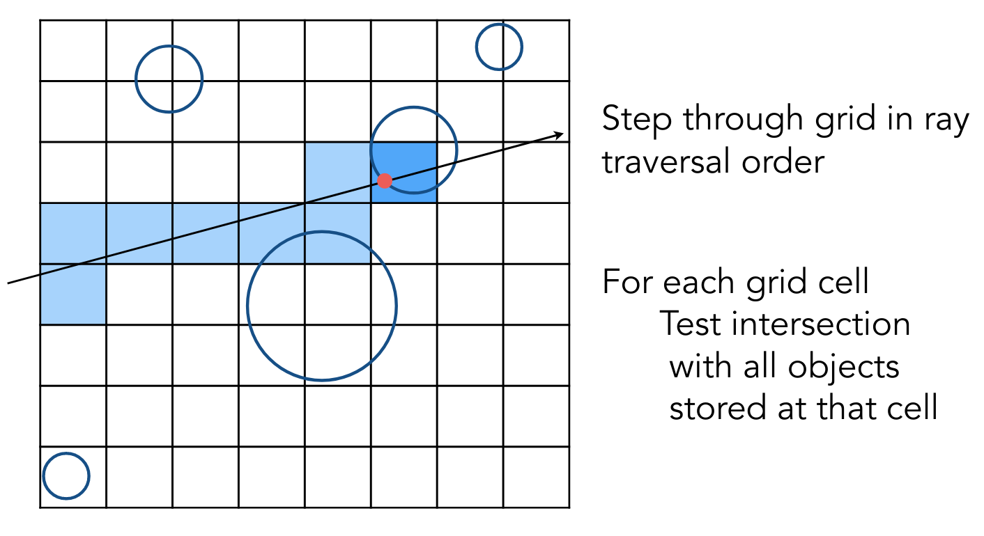
光线进行 grid traversal 时,不必考虑所有的 grids
以图中的方向为例,只需要考虑右面和上面的 grid 即可
类似画一条直线,参见 PA1 rasterizer.cpp 中的 draw_line 函数
Bresenham’s line drawing algorithm
对于 grid 的分辨率,若太大,起不到加速效果,若太小,光线与 grid 求交的开销太大
有经验规则
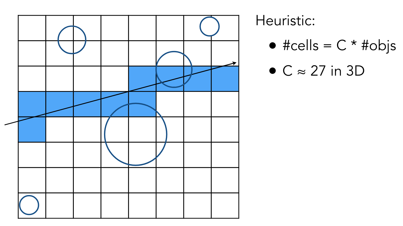
然而,均匀划分对于物体不均匀分布的场景而言效果并不好
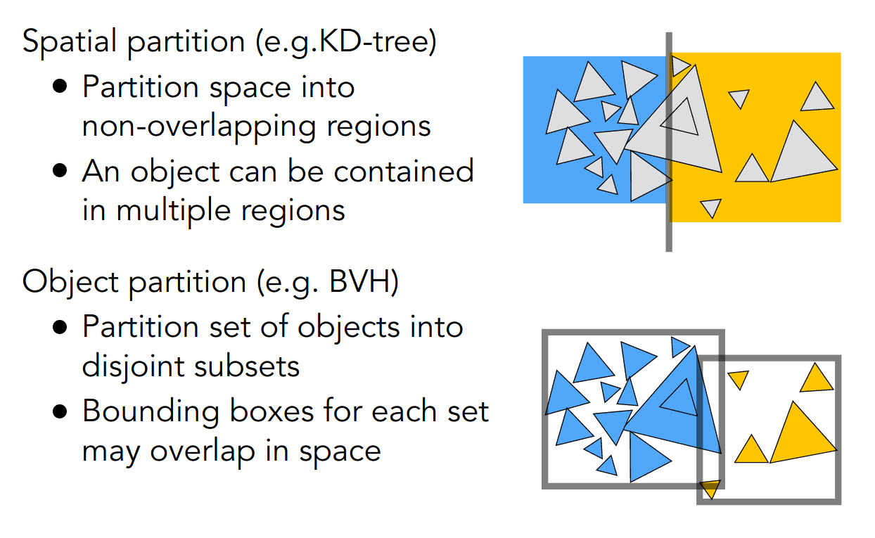
Spatial Partitions
考虑场景的不均匀划分
以 KD-Tree 为例,region 构成一个二叉树
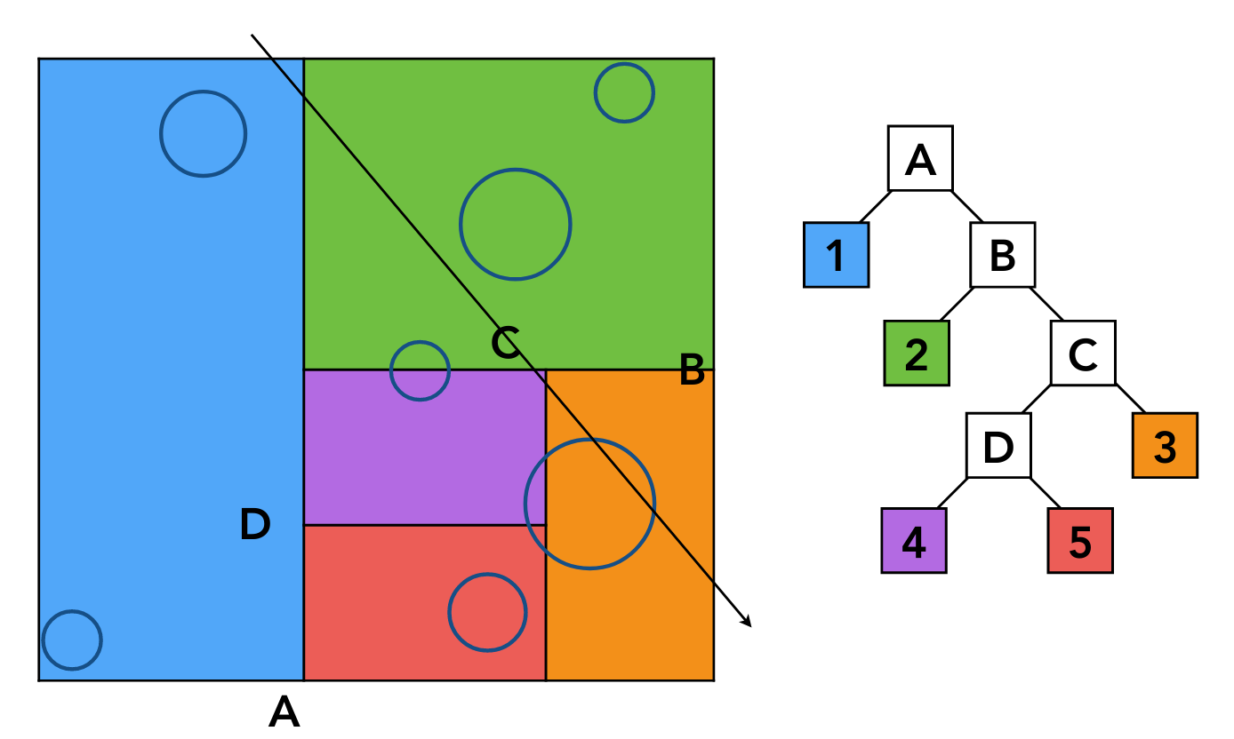
需要注意,叶子节点需要根据 region 计算哪些物体在其内部,这并不容易
并且物体可能同时在不同的 region 中
Object Partitions & Bounding Volume Hierarchy (BVH)
考虑物体的不均匀划分
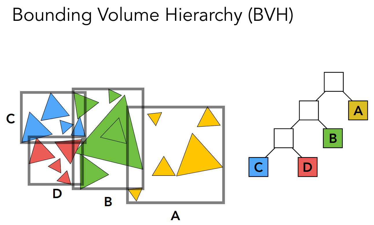
注意 Bounding Volumes 之间可能有重叠
每一次划分后,都需要重新计算子结构的 Bounding Volumes
而对于物体的划分,可以根据某个方向取中位数
总结一下求交的算法
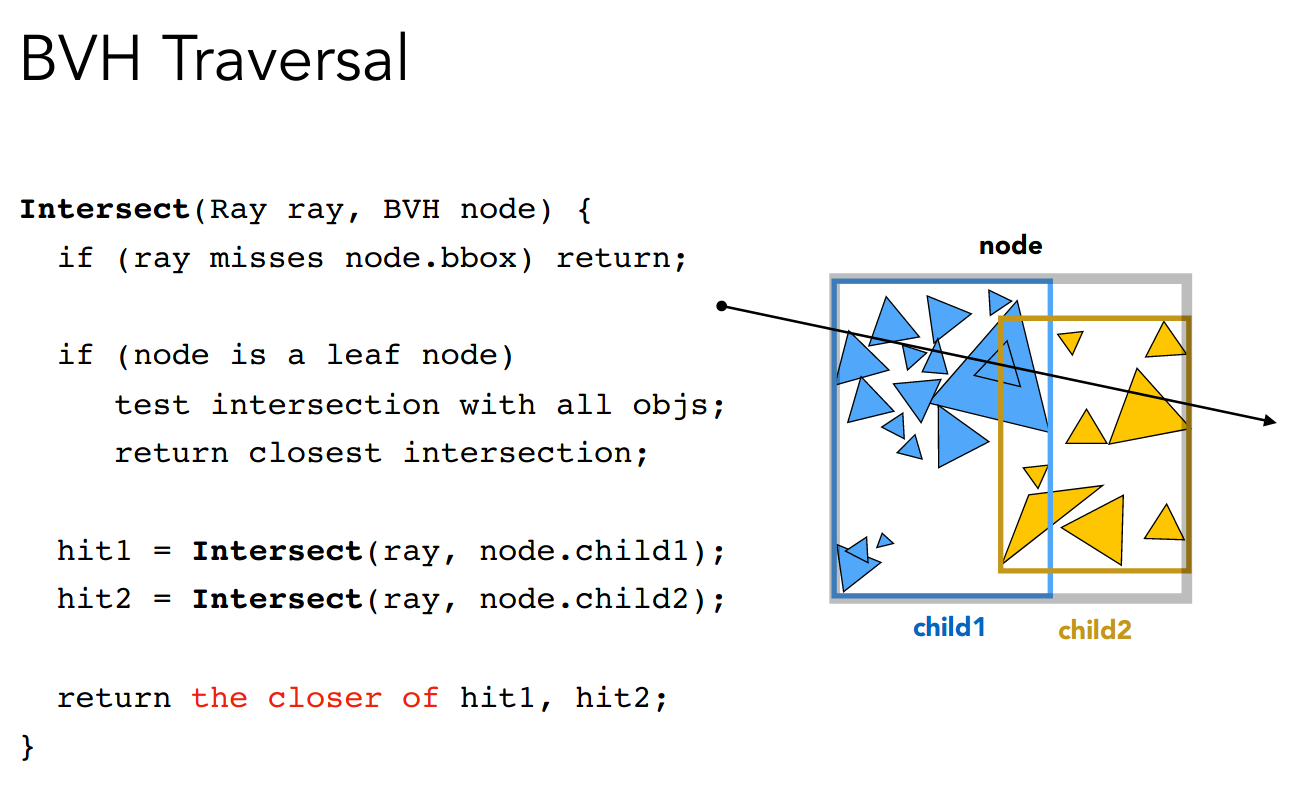
综合了
- 光线和 Surface 求交
- 光线和 Bounding Volume 求交
- 加速结构
区分一下上述两种不均匀划分
至此,Recursive (Whitted-Style) Ray Tracing 基本上就介绍完了
Basic Radiometry
进入辐射度量学这个新的话题
我们需要对光的空间特性进行更精确的度量
首先引入几个概念
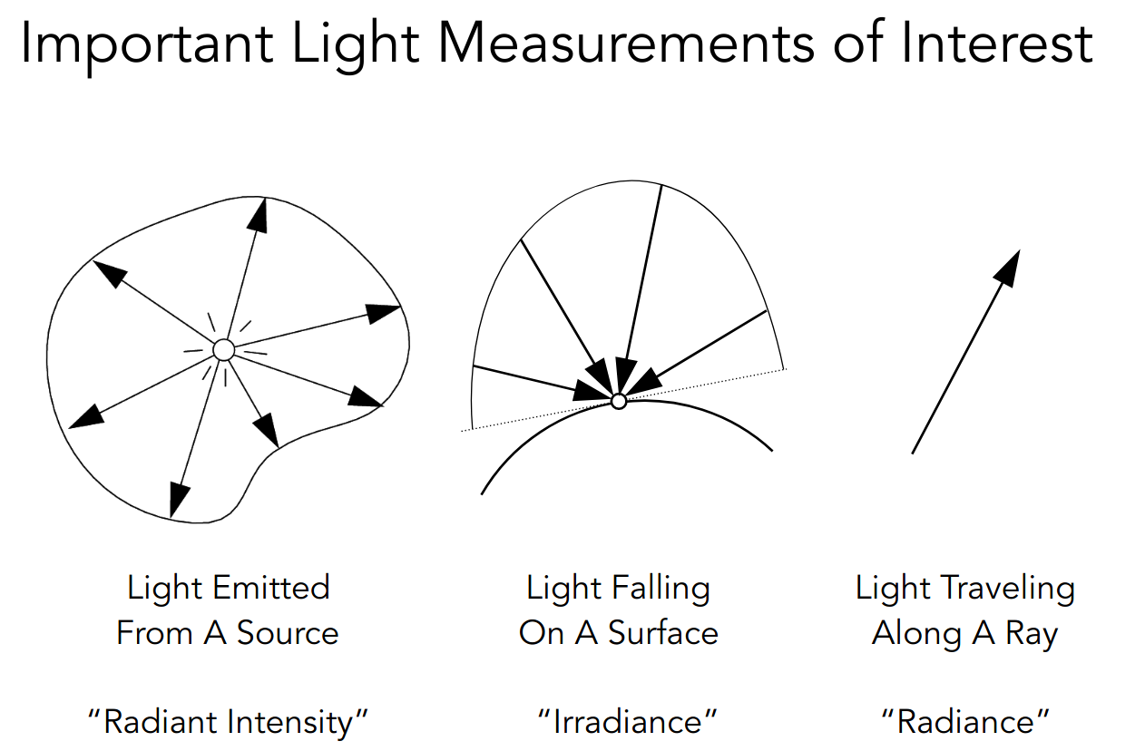
Radiant Energy
能量 - 焦耳
Radiant Flux (Power)
功率/辐射通量 - 瓦特/流明
Radiant Intensity
辐射强度 - 坎德拉
其中 为立体角
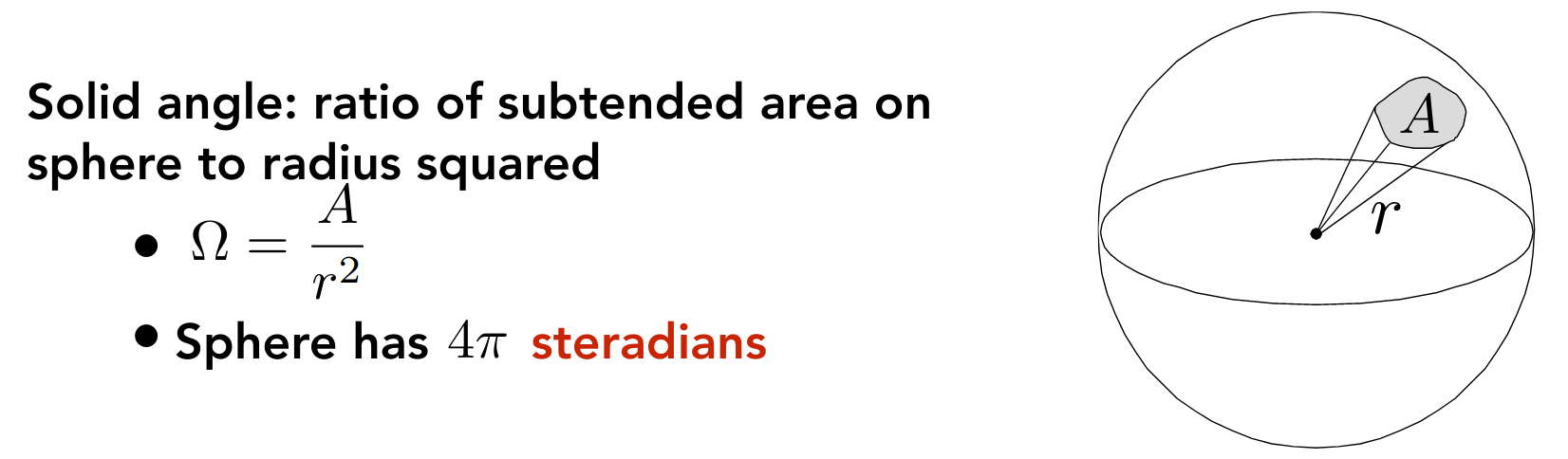
加上微分符号就是微分立体角,即球面空间中一个方向上的单位立体角
使用球坐标系易知
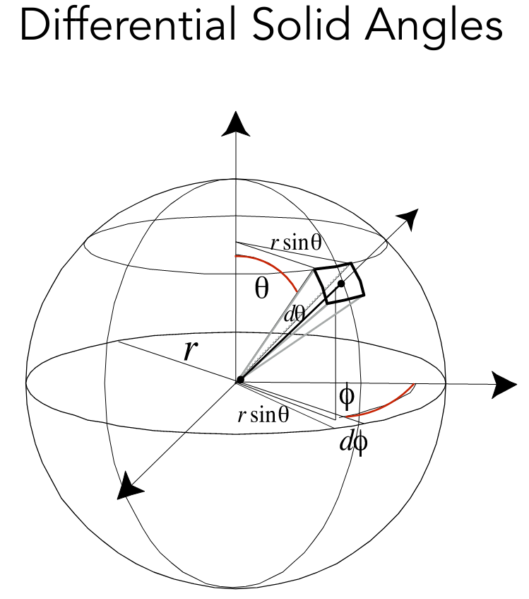
于是 Radiant Flux 和 Radiant Intensity 有关系
PA6
使用 Bounding Volumes 加速光线追踪
migration
首先需要将 PA5 的代码迁移过来
PA6 抽象出了 Scene 类和 Ray 类
castRay 的调用方式有所改变
  for (uint32_t j = 0; j < scene.height; ++j) {    for (uint32_t i = 0; i < scene.width; ++i) {      // generate primary ray direction      float x =          (2 * (i + 0.5) / (float)scene.width - 1) * imageAspectRatio * scale;      float y = (1 - 2 * (j + 0.5) / (float)scene.height) * scale;      // TODO: Find the x and y positions of the current pixel to get the      // direction vector that passes through it.      // Also, don't forget to multiply both of them with the variable      // *scale*, and x (horizontal) variable with the *imageAspectRatio*
      Vector3f dir = normalize(          Vector3f(x, y, -1)); // Don't forget to normalize this direction!      framebuffer[m++] = scene.castRay(Ray{eye_pos, dir}, 0);    }    UpdateProgress(j / (float)scene.height);  }
然后需要修改 Triangle.hpp 中的 getIntersection
inline Intersection Triangle::getIntersection(Ray ray) {  Intersection inter;
  if (dotProduct(ray.direction, normal) > 0)    return inter;  double u, v, t_tmp = 0;  Vector3f pvec = crossProduct(ray.direction, e2); // s1  double det = dotProduct(e1, pvec);  if (fabs(det) < EPSILON)    return inter;
  double det_inv = 1. / det;  Vector3f tvec = ray.origin - v0; // s  u = dotProduct(tvec, pvec) * det_inv;  if (u < 0 || u > 1)    return inter;  Vector3f qvec = crossProduct(tvec, e1); // s2  v = dotProduct(ray.direction, qvec) * det_inv;  if (v < 0 || u + v > 1)    return inter;  t_tmp = dotProduct(e2, qvec) * det_inv;
  // TODO find ray triangle intersection  if (t_tmp < 0)    return inter;
  inter.happened = true;  inter.coords = ray(t_tmp);  inter.distance = std::min(inter.distance, t_tmp); // dir is normalized  // assume  inter.normal = normal;  inter.obj = (Object *)this;  inter.m = m;
  return inter;}
Triangle 类和 MeshTriangle 类 override 掉 getIntersection 方法
但是 MeshTriangle 类的实现和 Triangle 类的实现并不一致
MeshTriangle 类需要调用
BVHAccel::Intersect
可能是因为 Triangle 类代表了 Implicit Surfaces,而 MeshTriangle 类代表了 Explicit Surfaces
还有一些奇怪的 intersect 方法,似乎并没有被使用
Bounds3::IntersectP
然后实现光线和 Bounding Volumes 求交
inline bool Bounds3::IntersectP(const Ray &ray, const Vector3f &invDir,                                const std::array<int, 3> &dirIsNeg) const {  // invDir: ray direction(x,y,z), invDir=(1.0/x,1.0/y,1.0/z),  // use this because Multiply is faster that Division  // dirIsNeg: ray direction(x,y,z), dirIsNeg=[int(x>0),int(y>0),int(z>0)],  // use this to simplify your logic
  // TODO test if ray bound intersects  double tx_min = (pMin.x - ray.origin.x) * invDir.x;  double tx_max = (pMax.x - ray.origin.x) * invDir.x;  if (tx_min > tx_max)    std::swap(tx_min, tx_max);
  double ty_min = (pMin.y - ray.origin.y) * invDir.y;  double ty_max = (pMax.y - ray.origin.y) * invDir.y;  if (ty_min > ty_max)    std::swap(ty_min, ty_max);
  double tz_min = (pMin.z - ray.origin.z) * invDir.z;  double tz_max = (pMax.z - ray.origin.z) * invDir.z;  if (tz_min > tz_max)    std::swap(tz_min, tz_max);
  double t_enter = std::max({tx_min, ty_min, tz_min});  double t_exit = std::min({tx_max, ty_max, tz_max});
  return t_enter < t_exit && t_exit >= 0;}
由于平面是和坐标轴是平行的,所以 Bounds3 类中存储了三对平面的某个轴的坐标
例如平行于 yz 平面的平面只需要存储 x 坐标
另外需要保证
并没有使用 dirIsNeg 参数
BVHAccel::getIntersection
最后实现利用加速结构的求交的算法
Intersection BVHAccel::getIntersection(BVHBuildNode *node,                                       const Ray &ray) const {  // TODO Traverse the BVH to find intersection  if (!node->bounds.IntersectP(          ray, ray.direction_inv,          std::array<int, 3>{static_cast<int>(ray.direction.x > 0),                             static_cast<int>(ray.direction.y > 0),                             static_cast<int>(ray.direction.z > 0)})) {    return Intersection{};  }
  // leaf node  if (!node->left and !node->right) {    return node->object->getIntersection(ray); // one object  }
  assert(node->left and node->right);
  Intersection l_isect = getIntersection(node->left, ray);  Intersection r_lsect = getIntersection(node->right, ray);
  return (l_isect.distance < r_lsect.distance) ? l_isect : r_lsect;}
注意到每个叶子节点,也就是每个 Bounding Volume 中只有一个物体
可以通过 BVHAccel::recursiveBuild 观察建立 BVH 的细节
总结一下调用轨迹
Scene::castRayScene::intersectBVHAccel::IntersectBVHAccel::getIntersectionBounds3::IntersectP
pic
todo
- Surface Area Heuristic
光线追踪(辐射度量学、渲染方程与全局光照)
Basic Radiometry
接着上节课的内容
Irradiance
辐射照度 - 勒克斯
注意这里的面积是投影面积
Radiance
辐射亮度
比 Irradiance 相比多了一个方向
比 Intensity 相比多了一个面积
power per unit solid angle per projected unit area
请关注如下的关系
- Irradiance: power per projected unit area
- Intensity: power per solid angle
- Radiance: Irradiance per solid angle
- Radiance: Intensity per projected unit area
于是有
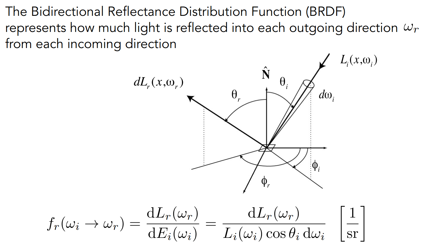
Bidirectional Reflectance Distribution Function (BRDF)
本质上是一个比例
The Reflection Equation
对半球面所有可能的方向积分即可
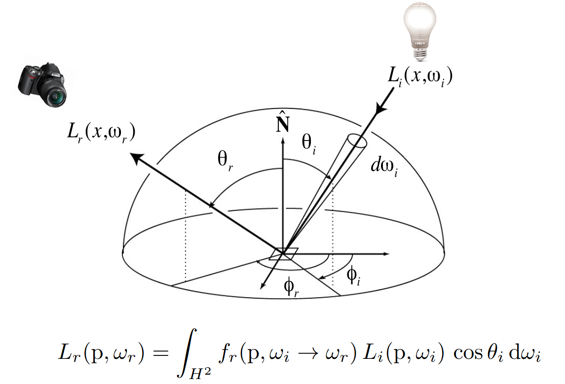
The Rendering Equation
加上着色点本身的辐射,即 Emission 项
代表半球面
we assume that all directions are pointing outwards
需要理解 Reflection 项积分符号的含义
当只有一个点光源时
当有多个点光源时,求和即可
当光源有一定的大小,即非点光源时,积分即可
为了处理多次反射的情形,我们视反射光也为光源,将等式简化为
考虑全局性,继续简化为
are vectors, is the light transport matrix
可以解得
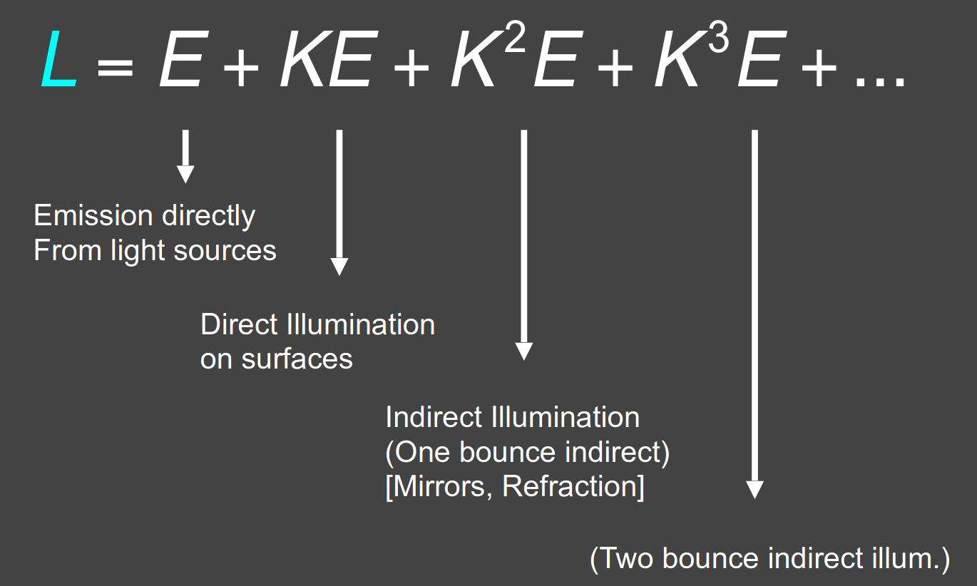
注意之前所学的光栅化着色的 Shadow Mapping 只能计算前两项
除了第一项,其余部分即为 global illumination 全局光照
光线追踪(蒙特卡洛积分与路径追踪)
Monte Carlo Integration
数值方法求近似积分
是连续型随机变量
以均匀分布为例,,则
Path Tracing
Whitted-Style Ray Tracing 有如下假设
- Always perform specular reflections / refractions
- Stop bouncing at diffuse surfaces
然而这些假设并不合理
为此我们需要借助上节课的 The Rendering Equation 进行光线追踪
考虑计算全局光照,对于给定的着色点和观察方向
利用蒙特卡洛积分,有如下的算法
shade(p, wo) Randomly choose N directions wi~pdf Lo = 0.0 For each wi Trace a ray r(p, wi) If ray r hit the light Lo += (1 / N) * L_i * f_r * cosine / pdf(wi) Else If ray r hit an object at q Lo += (1 / N) * shade(q, -wi) * f_r * cosine / pdf(wi) Return Lo注意这里的
第一个分支计算直接光照,即第二项
第二个分支使用递归计算所有的间接光照,即第二项之后的项
注意对 取反方向
但需要注意这里递归会爆炸,有关系 rays = N ^ bounces
所以我们取 N = 1
shade(p, wo) Randomly choose ONE direction wi~pdf(w) Trace a ray r(p, wi) If ray r hit the light Return L_i * f_r * cosine / pdf(wi) Else If ray r hit an object at q Return shade(q, -wi) * f_r * cosine / pdf(wi)但随机性引入了噪声,所以我们需要在 ray_generation 时取 N 个方向
ray_generation(camPos, pixel) Uniformly choose N sample positions within the pixel pixel_radiance = 0.0 For each sample in the pixel Shoot a ray r(camPos, cam_to_sample) If ray r hit the scene at p pixel_radiance += 1 / N * shade(p, sample_to_cam) Return pixel_radianceSPP (samples per pixel)
然而上述着色算法仍存在问题,即递归可能不会终止
为此引入 Russian Roulette,即俄罗斯轮盘赌
- 设定某个概率
- 概率下,计算着色并将最终结果除以
- 概率下,直接返回结果
这可以保证最终结果的期望相同
shade 算法如下
shade(p, wo)    Manually specify a probability P_RR    Randomly select ksi in a uniform dist. in [0, 1]    If (ksi > P_RR) return 0.0;
Randomly choose ONE direction wi~pdf(w) Trace a ray r(p, wi) If ray r hit the light Return L_i * f_r * cosine / pdf(wi) / P_RR Else If ray r hit an object at q Return shade(q, -wi) * f_r * cosine / pdf(wi) / P_RR另外注意到,当光源较小时,shade 追踪的光线可能很难 hit 光源
为此考虑在光源平面,而非在着色点平面,进行采样
需要对 进行变换
sample on x, integrate on x
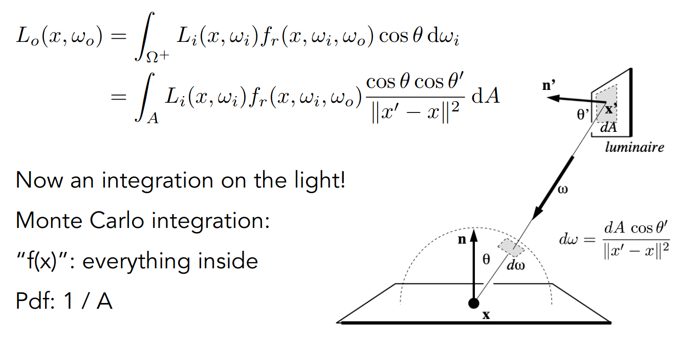
于是将着色分为两个部分
- light source (direct, no need to have RR)
- other reflectors (indirect, RR)
shade 算法最终如下
shade(p, wo)    # Contribution from the light source.    Uniformly sample the light at x’ (pdf_light = 1 / A)  Shoot a ray from p to x’  If the ray is not blocked in the middle    L_dir = 0.0  Else    L_dir = L_i * f_r * cos θ * cos θ’ / |x’ - p|^2 / pdf_light
    # Contribution from other reflectors.    L_indir = 0.0    Test Russian Roulette with probability P_RR    Uniformly sample the hemisphere toward wi (pdf_hemi = 1 / 2pi)    Trace a ray r(p, wi)    If ray r hit a non-emitting object at q      L_indir = shade(q, -wi) * f_r * cos θ / pdf_hemi / P_RR
    Return L_dir + L_indir
需要考虑到光源和着色点之间有 block 的情形
Further…
- Uniformly sampling the hemisphere
How? And in general, how to sample any function? (sampling)
- Monte Carlo integration allows arbitrary pdfs
What’s the best choice? (importance sampling)
- Do random numbers matter?
Yes! (low discrepancy sequences)
- I can sample the hemisphere and the light
Can I combine them? Yes! (multiple imp. sampling)
- The radiance of a pixel is the average of radiance on all paths passing through it
Why? (pixel reconstruction filter)
- Is the radiance of a pixel the color of a pixel?
No. (gamma correction, curves, color space)
PA7
algorithm
伪代码如下
shade(p, wo)  L_dir = 0.0  sampleLight(inter, pdf_light)  Get x, ws, NN, emit from inter  Shoot a ray from p to x  If the ray is not blocked in the middle    L_dir = emit * eval(wo, ws, N) * dot(ws, N) * dot(ws, NN) / |x-p|^2 / pdf_light
  L_indir = 0.0  Test Russian Roulette with probability RussianRoulette  wi = sample(wo, N)  Trace a ray r(p, wi)  If ray r hit a non-emitting object at q    L_indir = shade(q, wi) * eval(wo, wi, N) * dot(wi, N) / pdf(wo, wi, N) / RussianRoulette
  Return L_dir + L_indir
实现如下
// Implementation of Path TracingVector3f Scene::castRay(const Ray &ray, int depth) const {  // TODO: Implement Path Tracing Algorithm here  Vector3f L_dir{};  Vector3f L_indir{};
  Intersection inter_wo = this->intersect(ray);
  if (!inter_wo.happened) {    return Vector3f{0};  }
  // direct  Vector3f wo = normalize(-ray.direction); // note negate  Vector3f p = inter_wo.coords;  Vector3f N = normalize(inter_wo.normal);
  Intersection inter_ws{};  float pdf_ws{};  this->sampleLight(inter_ws, pdf_ws);
  Vector3f x = inter_ws.coords;  Vector3f NN = normalize(inter_ws.normal);  Vector3f emit = inter_ws.emit;
  Vector3f ws = normalize(x - p);  Ray ray_p_to_x(p, ws);
  Intersection inter_p_to_x = this->intersect(ray_p_to_x);  // if (inter_p_to_x.happened && inter_p_to_x.obj->hasEmit()) { // assume  if (inter_p_to_x.happened && (inter_p_to_x.coords - x).norm() < 0.01) {    Vector3f eval_f_r = inter_wo.m->eval(ws, wo, N); // note order    L_dir = emit * eval_f_r * dotProduct(ws, N) *            dotProduct(-ws, NN) / // note negate            ((x - p).norm() * (x - p).norm() * pdf_ws);  } else {    // the ray is blocked in the middle    // do nothing  }
  // indirect  if (get_random_float() < this->RussianRoulette) {    Vector3f wi = normalize(inter_wo.m->sample(wo, N));    Ray ray_wi(p, wi);    // Intersection intersection_wi = this->intersect(ray_wi);    // if (intersection_wi.happened && !intersection_wi.obj->hasEmit()) {    Vector3f shade = castRay(ray_wi, depth + 1);    Vector3f eval_f_r = inter_wo.m->eval(wi, wo, N); // note order    float pdf = inter_wo.m->pdf(wi, wo, N);    L_indir =        shade * eval_f_r * dotProduct(wi, N) / (pdf * this->RussianRoulette);    // }  } else {    // do nothing  }
  return L_dir + L_indir;}
note
修改 Bounds3::IntersectP 中的相交条件
t_enter <= t_exit && t_exit >= 0多一个等号
示意图如下

注意光线的方向,对 p 点而言,始终是 outwards
区分 eval 和 pdf 中的参数 wi 和 wo
关于检测光源和着色点之间是否有 block,需要射出额外的光线 ray_p_to_x,并判断交点和 x 点是否一致
关于间接光照,似乎并不需要分支判断
参数 depth 代表递归的次数,不过没有用到
thread
参考 https://github.com/Quanwei1992/GAMES101/blob/master/07/Renderer.cpp
使用多线程加速渲染,按 height 将屏幕划分给多个 worker
并且修改 CMakeLists.txt
find_package(Threads REQUIRED)target_link_libraries(RayTracing PUBLIC Threads::Threads)速度提升了约 2~3 倍
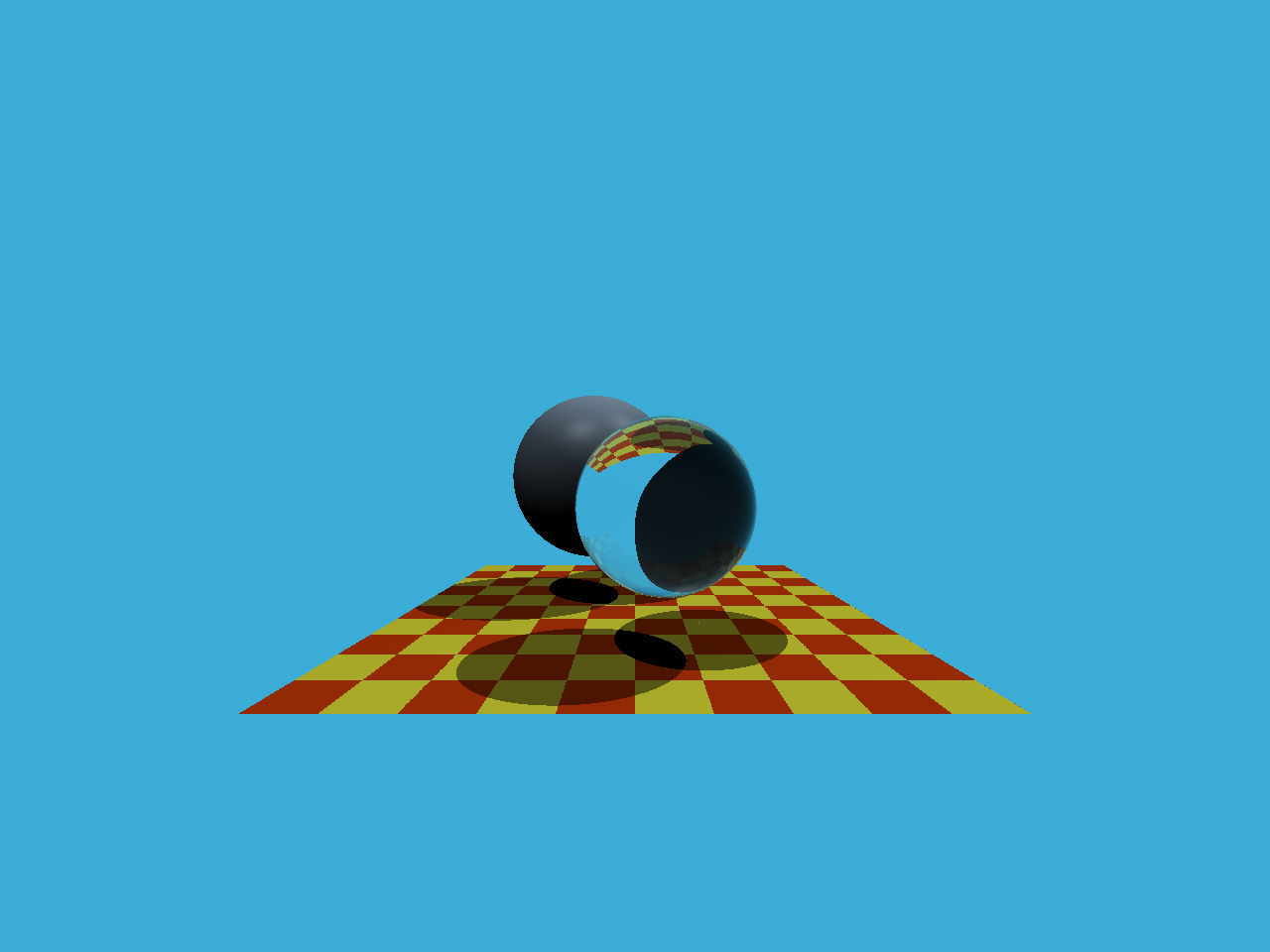
pic
128 spp
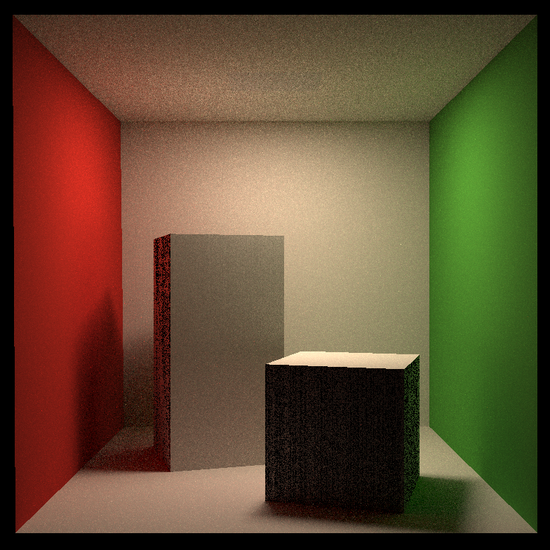
渲染了一个小时
todo
- 使光源可见
TODO
图形学对其他学科的要求挺高的……
而且调试完全没有头绪……
于是就这样吧……