TOC
Open TOC
- Info
- Ref
- Intro
- IR
- DFA-AP
- A1
- DFA-FD
- Understand the functional view of iterative algorithm
- The definitions of lattice and complete lattice
- Understand the fixed-point theorem
- How to summarize may and must analyses in lattices
- The relation between MOP and the solution produced by the iterative algorithm
- Constant propagation analysis
- Worklist algorithm
- A2
- A3
- Inter
- A4
- PTA
- PTA-FD
- A5
- PTA-CS
- Concept of context sensitivity (C.S.)
- Concept of context-sensitive heap (C.S. heap)
- Why C.S. and C.S. heap improve precision
- Context-sensitive pointer analysis rules
- Algorithm for context-sensitive pointer analysis
- Common context sensitivity variants
- Differences and relationship among common context sensitivity variants
- Call-Site vs. Object Sensitivity
- A6
- A7
- Security
- A8
Info
https://pascal-group.bitbucket.io/teaching.html
Ref
https://github.com/pascal-lab/Tai-e-assignments/issues/2
https://github.com/DianQK/Tai-e-assignments-tips
https://github.com/RicoloveFeng/SPA-Freestyle-Guidance
Intro
What are the differences between static analysis and (dynamic) testing?
在程序执行前分析程序是否满足一些不平凡的性质,如是否存在内存泄漏
根据 Rice’s Theorem,对于现代编程语言而言,对于这些问题无法给出确切的答案
(recursively enumerable) = recognizable by a Turing-machine
Understand soundness, completeness, false negatives, and false positives.
为此需要妥协,有两个方向,误报和漏报
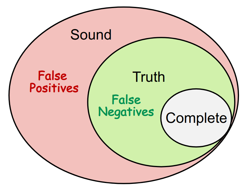
对于大部分静态分析而言,主要追求 sound
Why soundness is usually required by static analysis?
类 继承了类
考虑如下一段程序
if (...) {  B b = new B();  a.fld = b;} else {  C c = new C();  a.fld = c;}
B b’ = (B) a.fld;
在某种执行路径下是不正确的强制类型转换
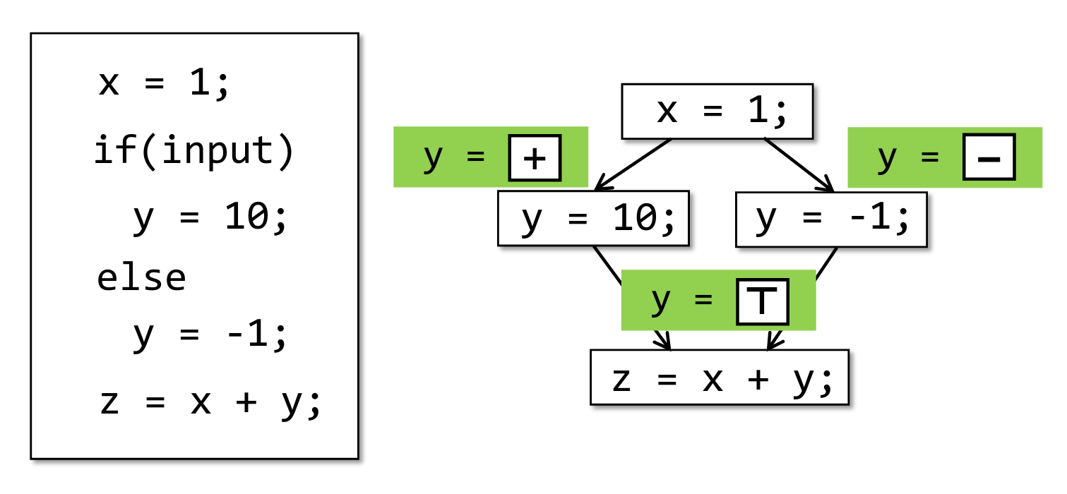
How to understand abstraction and over-approximation?
抽象
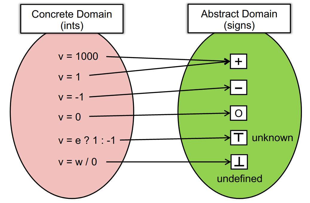
转换函数
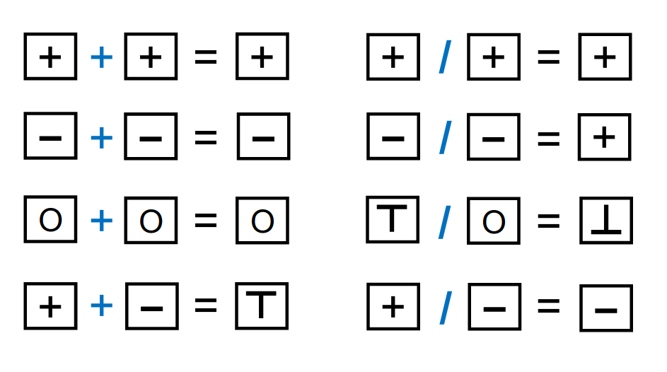
分支合并
IR
参考龙书
The relation between compilers and static analyzers
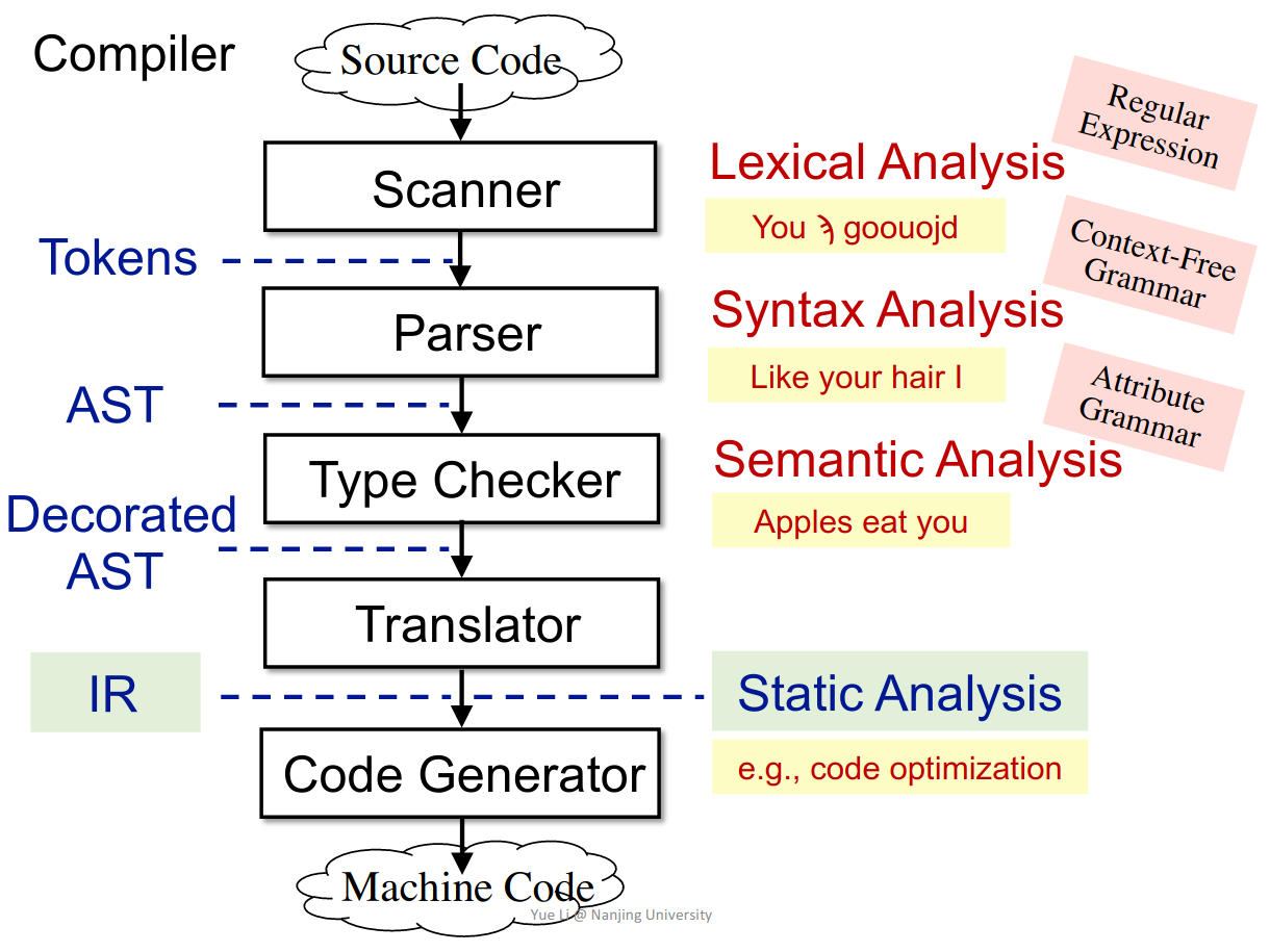
代码优化的部分
Understand 3AC and its common forms
三地址代码 3AC
静态单赋值 SSA
How to build basic blocks on top of IR
基本块
How to construct control flow graphs on top of BBs?
流图
DFA-AP
数据流分析 - 应用部分
参考龙书
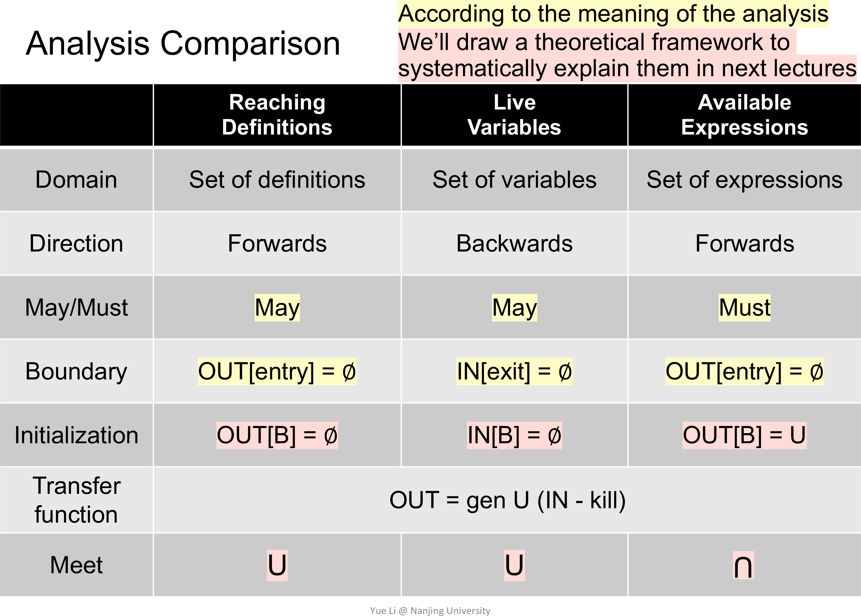
Understand the three data flow analyses
Reaching Definitions Analysis
在程序的某个点,哪些语句的定义仍然可达
考虑所有可能的执行路径,因而为 may analysis
可能的应用,检测未定义先使用
Live Variables Analysis
在程序的某个点,哪些变量在之后仍会被使用
为 may analysis
通过 out 求 in
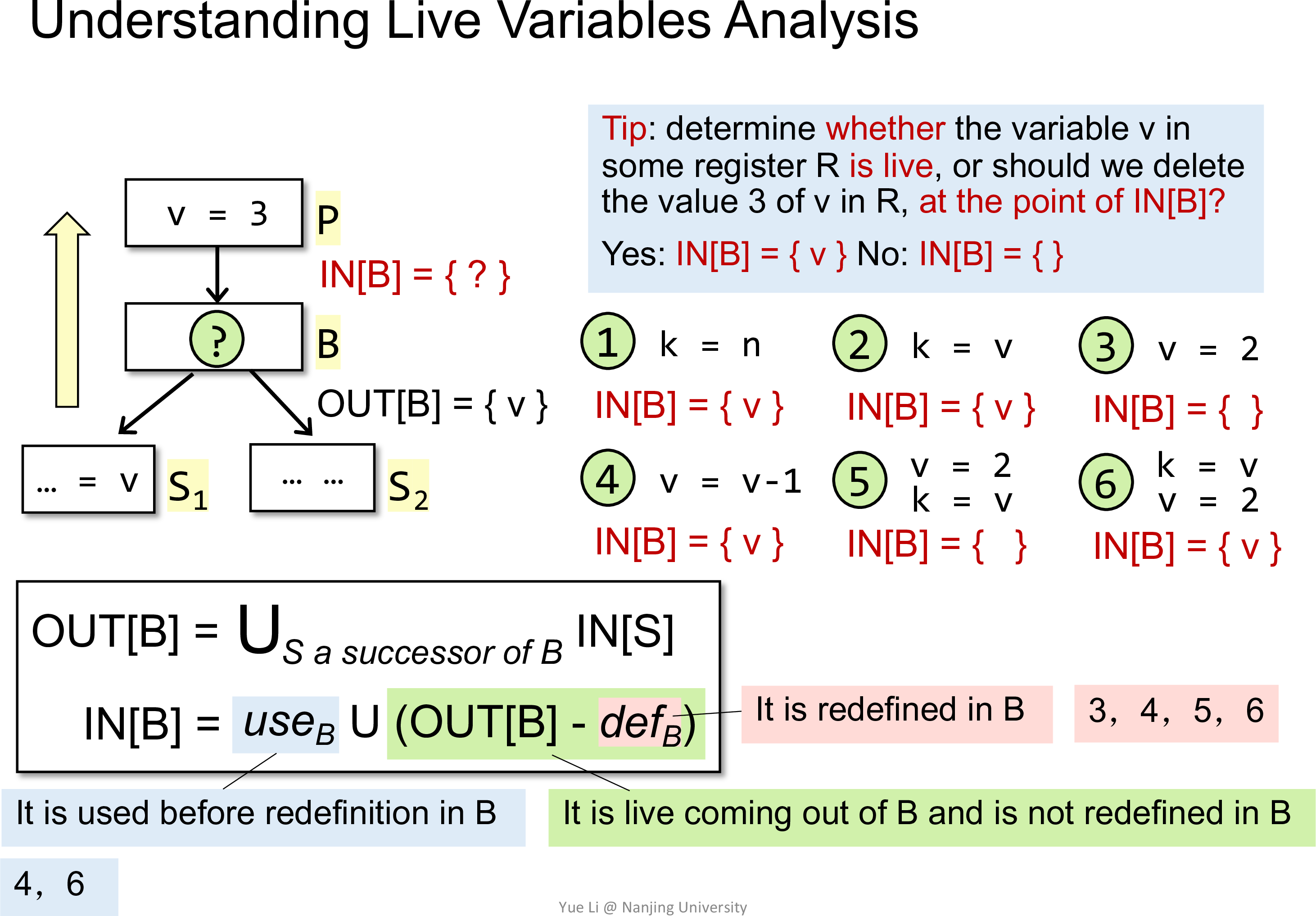
注意 define 前的 use 是算的
可能的应用,寄存器分配
Available Expressions Analysis
哪些表达式在所有的到达某个点的执行路径上都会被求值,且求值后没有出现再赋值
为 must analysis
可能的应用,寻找全局公共子表达式
Can tell the differences and similarities of the three data flow analyses
Understand the iterative algorithm and can tell why it is able to terminate
以 Reaching Definitions Analysis 为例
关注转移函数,gen 和 kill 固定
out 的基数不减,而 out 为有限集
所以当 out 不变时,即为不动点,算法停止
理论部分会给出严谨的说明
A1
主要参考这张图
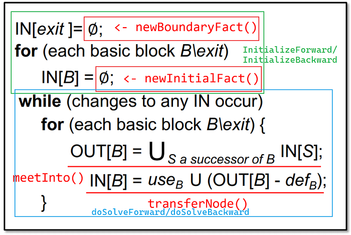
需要注意通用框架和具体策略的解耦
比如对于 LiveVariableAnalysis,newBoundaryFact 和 newInitialFact 直接返回一个空集即可
而不必考虑等号的左侧是 in 还是 out,是 exit 还是 node
这些内容是由 DataflowResult 类管理的
压缩命令
$ zip -j 201250012.zip src/main/java/pascal/taie/analysis/dataflow/analysis/LiveVariableAnalysis.java src/main/java/pascal/taie/analysis/dataflow/solver/IterativeSolver.java src/main/java/pascal/taie/analysis/dataflow/solver/Solver.javaDFA-FD
数据流分析 - 理论部分
Understand the functional view of iterative algorithm
将某次迭代后所有 node 的 domain 捆绑为一个元组
一次迭代就是对元组进行某种映射
实际上每个 node 的 domain 就是一个格
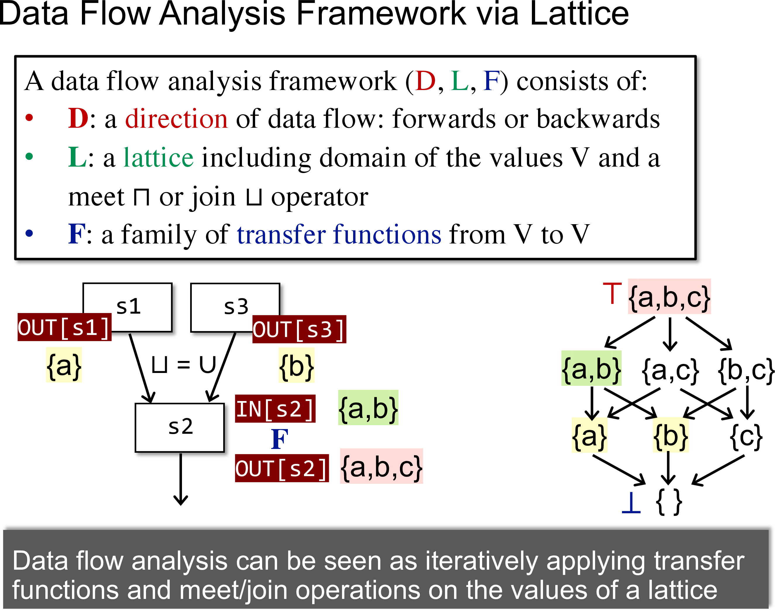
The definitions of lattice and complete lattice
lattice -> every pair of a poset’s elements has a least upper bound and a greatest lower bound
complete lattice -> all subsets of a lattice have a least upper bound and a greatest lower bound
least upper bound - join -
greatest lower bound - meet -
Understand the fixed-point theorem
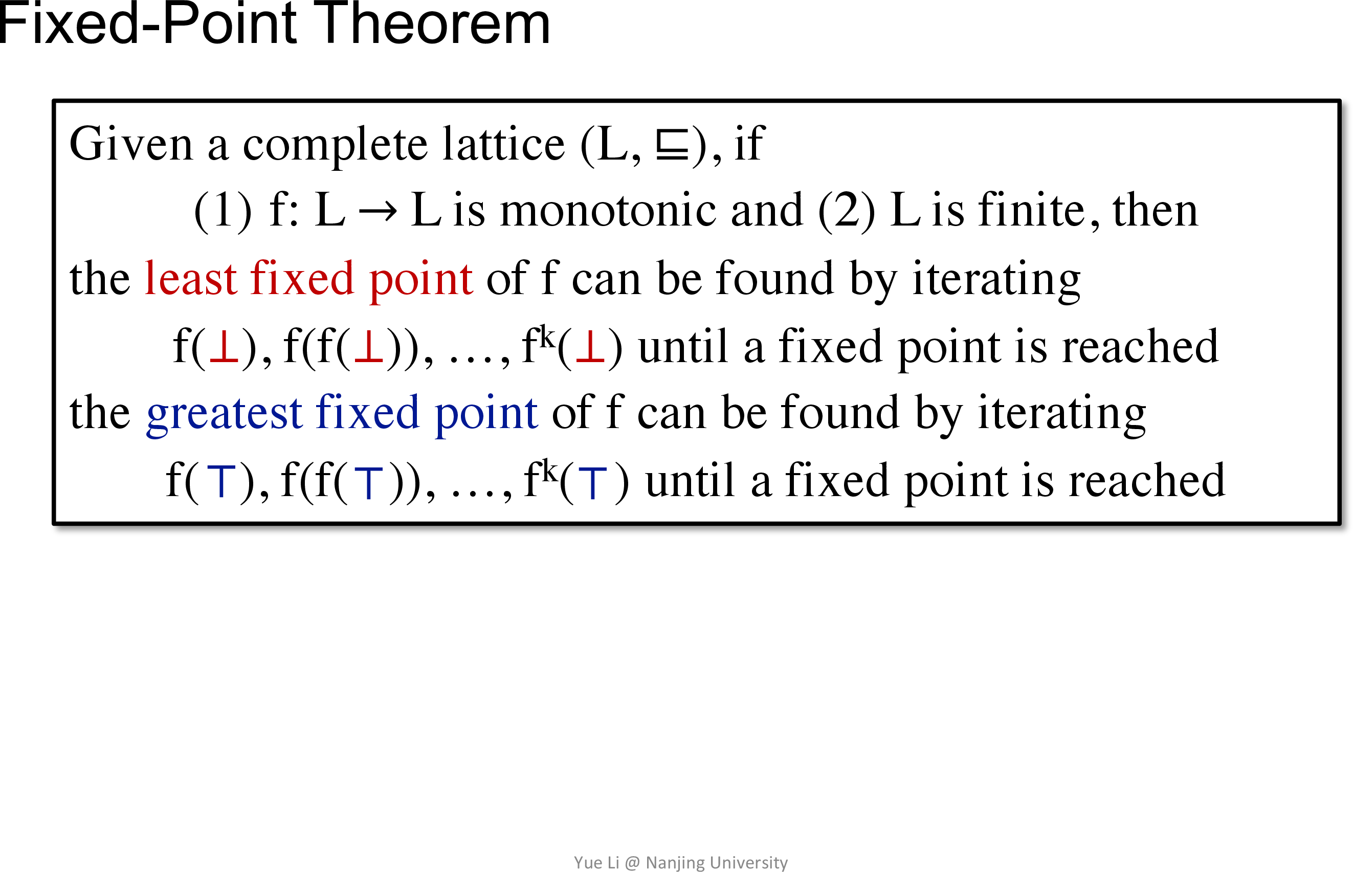
证明分为存在性和唯一性
由于是有限集,相当好证
How to summarize may and must analyses in lattices
首先需要用格的角度来看待数据流分析
然后需要关联 fixed-point theorem 和 dfa
实际上只要说明 transfer function 和 join/meet function 为单调
DFA-AP 已经说明了转移函数是不减的,又注意到
所以可以利用 fixed-point theorem 的结论得到
- iterative algorithm 会终止到一个不动点
- 该不动点为 least 或 greatest
下图解释了 may and must analyses
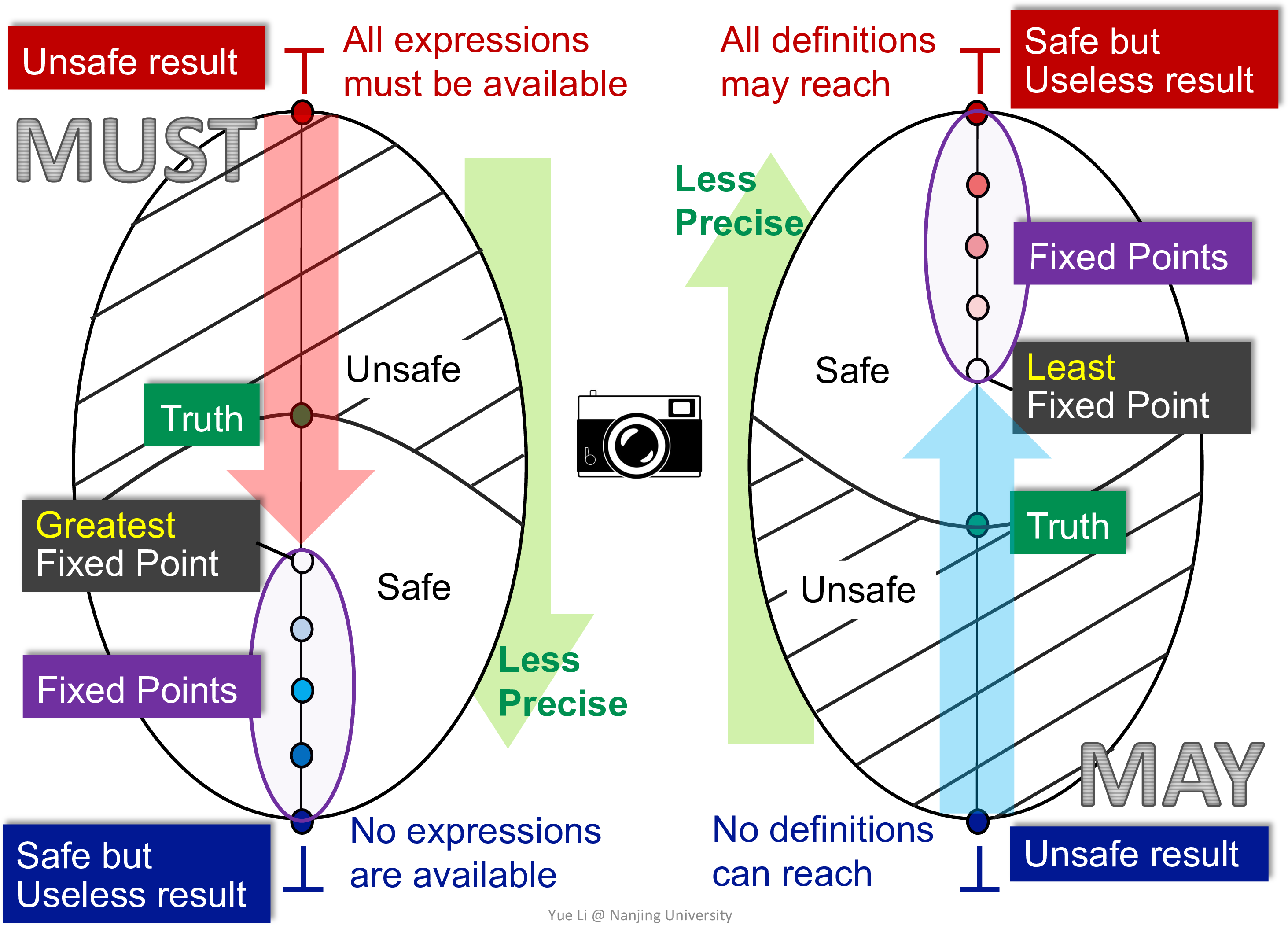
需要说明有如下几点
- may analyses 是查错用的,所以都是 1 最安全,即不能漏报
- must analyses 是优化用的,所以都是 0 最安全,即不能误报
- top 是极端激进,bottom 是极端保守
- 设计转移函数时,需要保证了不动点在 safe 区域中
The relation between MOP and the solution produced by the iterative algorithm
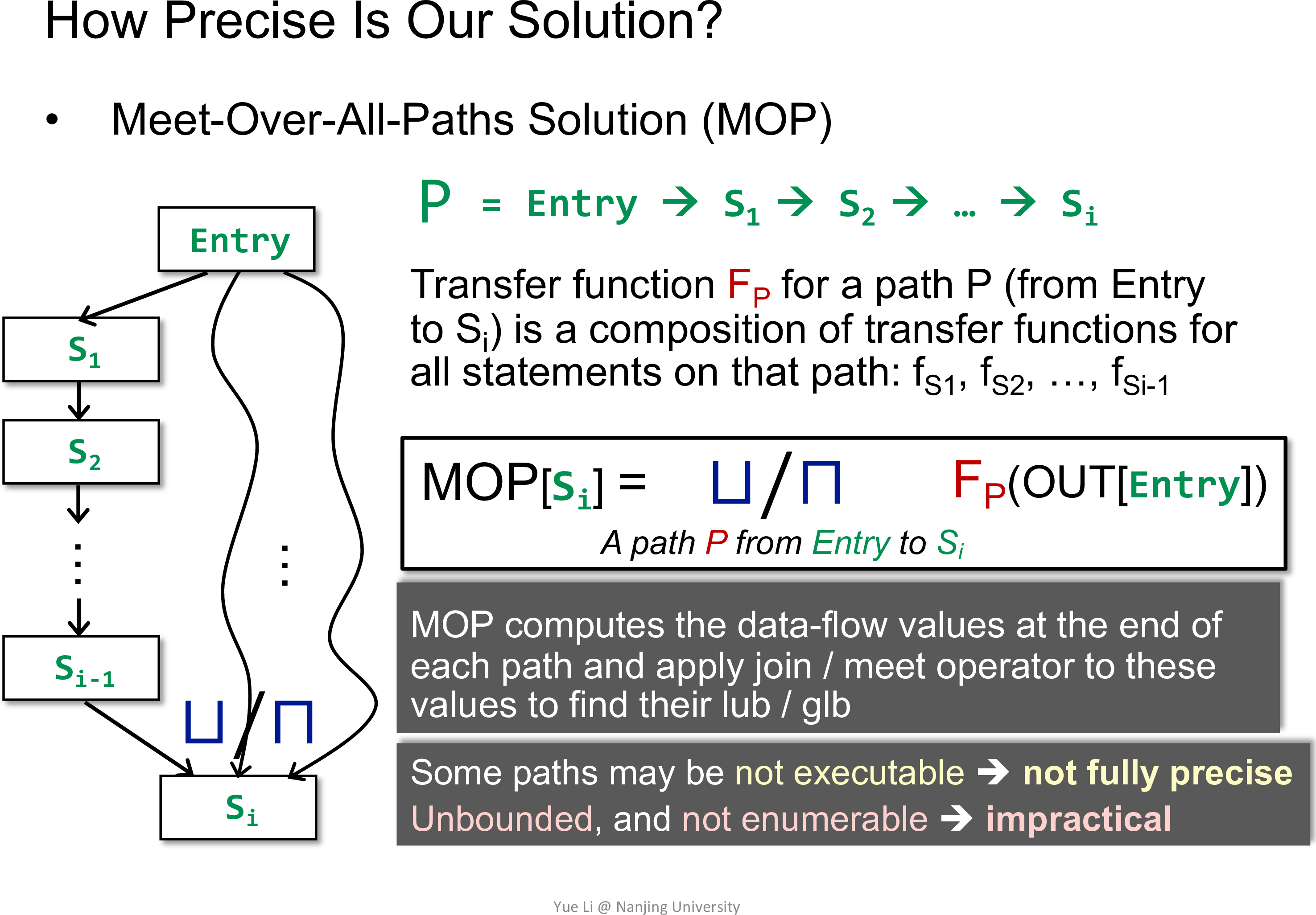
不难发现,iterative algorithm 为 ,而 MOP 为 ,其中 单调
注意到
等号成立当且仅当 为 distributive 的
所以 MOP 会更加精确
实际上在 DFA-AP 中 Bit-vector or Gen/Kill problems 的 都是 distributive 的
Constant propagation analysis
判断一个变量是否存储常量
具体见 A2
不为 distributive 的
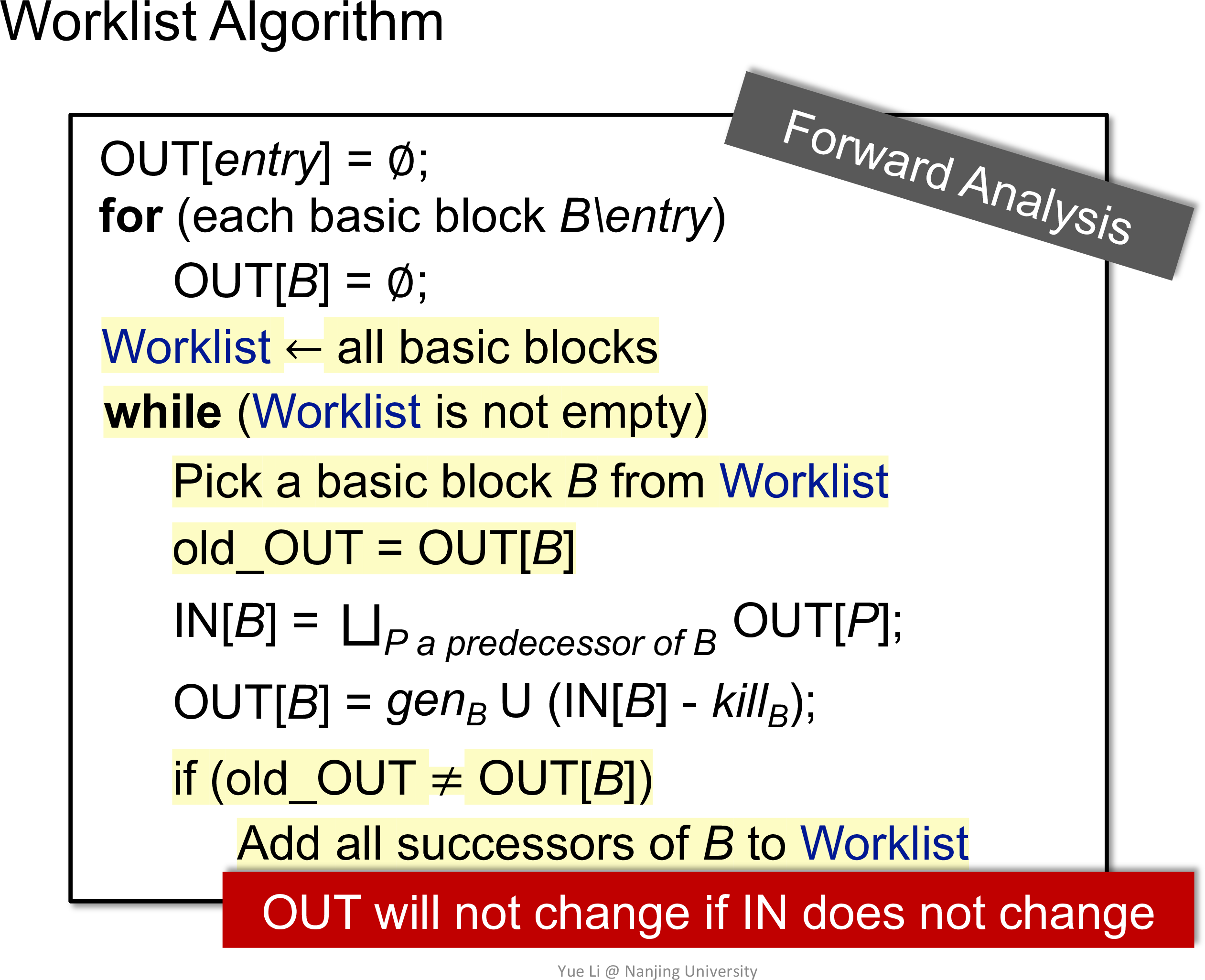
Worklist algorithm
优化 iterative algorithm,使用队列记录变化的 out 或 in
具体见 A2
A2
Constant propagation analysis
| constant propagation | |
|---|---|
| Domain | UNDEF / CONSTANT / NAC |
| Direction | Forwards |
| May/Must | Must - 优化 |
| Boundary | OUT[entry] = NAC for args |
| Initialization | OUT[B] = use absence to represent UNDEF |
| Transfer function | evaluate |
| Meet | meetValue |
Worklist algorithm
note
- 可以仿照 A1 的
doSolveBackward完成doSolveForward,完成 Constant propagation 后,再写 Worklist algorithm - 由于各个方法的分析可能是并发执行的,为了调试某个特定的方法,可以在内部使用条件断点
- 注意 CPFact 中对 UNDEF 的表示
submit
压缩命令
zip -j 201250012.zip src/main/java/pascal/taie/analysis/dataflow/analysis/constprop/ConstantPropagation.java src/main/java/pascal/taie/analysis/dataflow/solver/Solver.java src/main/java/pascal/taie/analysis/dataflow/solver/WorkListSolver.javaLoop.java发现 Worklist algorithm 写的有问题,fact 的变化应通过 transferNode 的返回值来判断BinaryOp.java发现evaluate有点问题,需要区分 UNDEF 和 NAC- 还有 7 个隐藏测试用例未通过……
A3
通过常量传播检测不可达代码
通过活跃变量分析检测无用赋值
注意 DeadCodeDetection 和 AbstractDataflowAnalysis 都继承了 MethodAnalysis
所以实际上 DeadCodeDetection 并未使用数据流分析的框架
但是其中使用了数据流分析的结果
虽然 A3 依赖于 A1 和 A2,但是 OJ 会提供正确的实现,所以即使 A2 没有完全通过也可以做 A3
压缩命令
zip -j 201250012.zip src/main/java/pascal/taie/analysis/dataflow/analysis/DeadCodeDetection.java总结一下关于 IR 的一些图
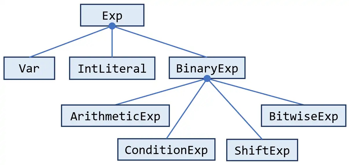
Subclasses of Exp
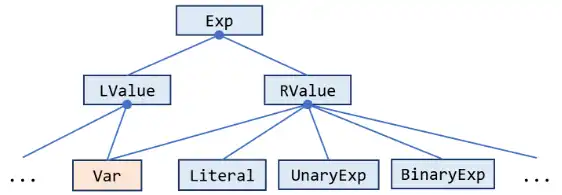
Subclasses of Exp
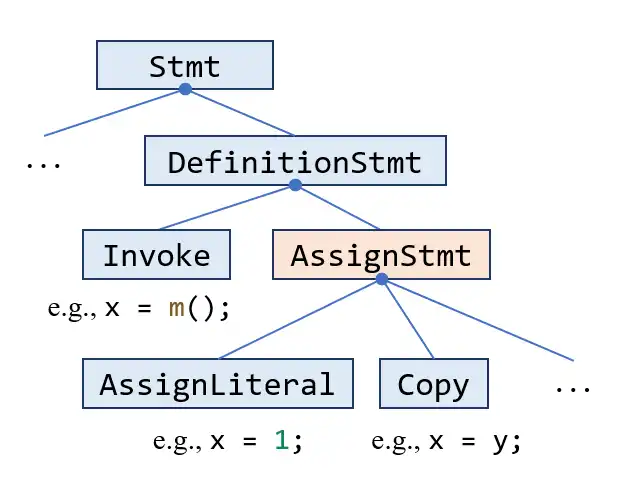
Subclasses of Stmt
Inter
How to build call graph via class hierarchy analysis
以面向对象语言 Java 为例
通过 CHA 构造调用图
也可以通过 pointer analysis 构造,效率较低但更精确
为此,需要了解 Java 的方法调用机制
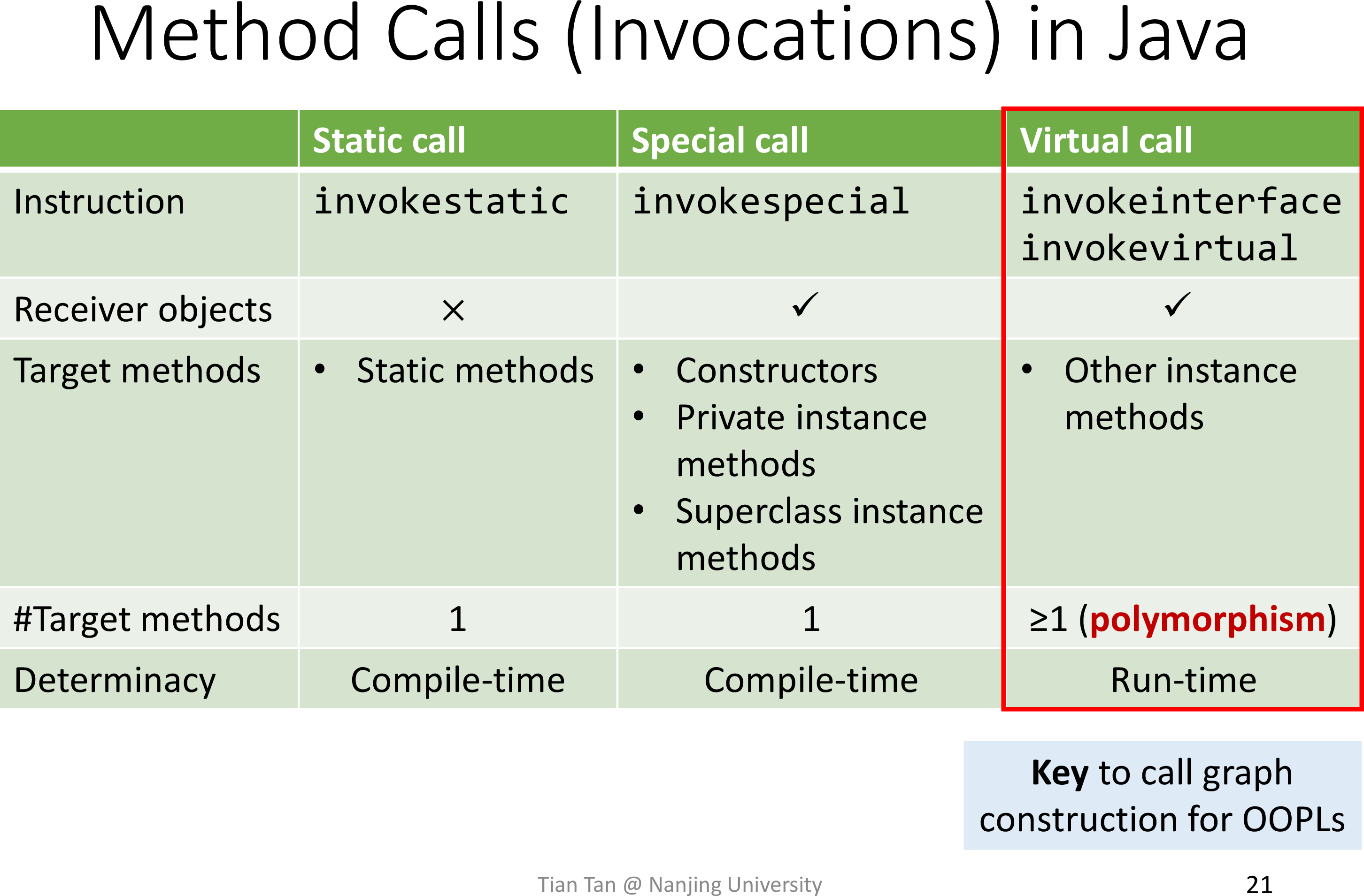
主要关注虚方法的分派 Dispatch
考虑如下代码
class A {    void foo() {…}}
class B extends A {}
class C extends B {    void foo() {…}}
void dispatch() {    A x = new B();    x.foo();    A y = new C();    y.foo();}
则有
Dispatch(B, A.foo()) = A.foo()Dispatch(C, A.foo()) = C.foo()direction -> superclass
对于方法的解析 Resolve 如下
- static call / sp call without super
- direct
- sp call with super / virtual call
- dispatch
- direction -> subclass
考虑如下代码
class A {    void foo() {…}}
class B extends A {}
class C extends B {    void foo() {…}}
class D extends B {    void foo() {…}}
void resolve() {    C c = …    c.foo();    A a = …    a.foo();    B b = …    b.foo();}
则有
Resolve(c.foo()) = {C.foo()}Resolve(a.foo()) = {A.foo(), C.foo(), D.foo()}Resolve(b.foo()) = {A.foo(), C.foo(), D.foo()}注意只关注 declared type,所以结果并不精确
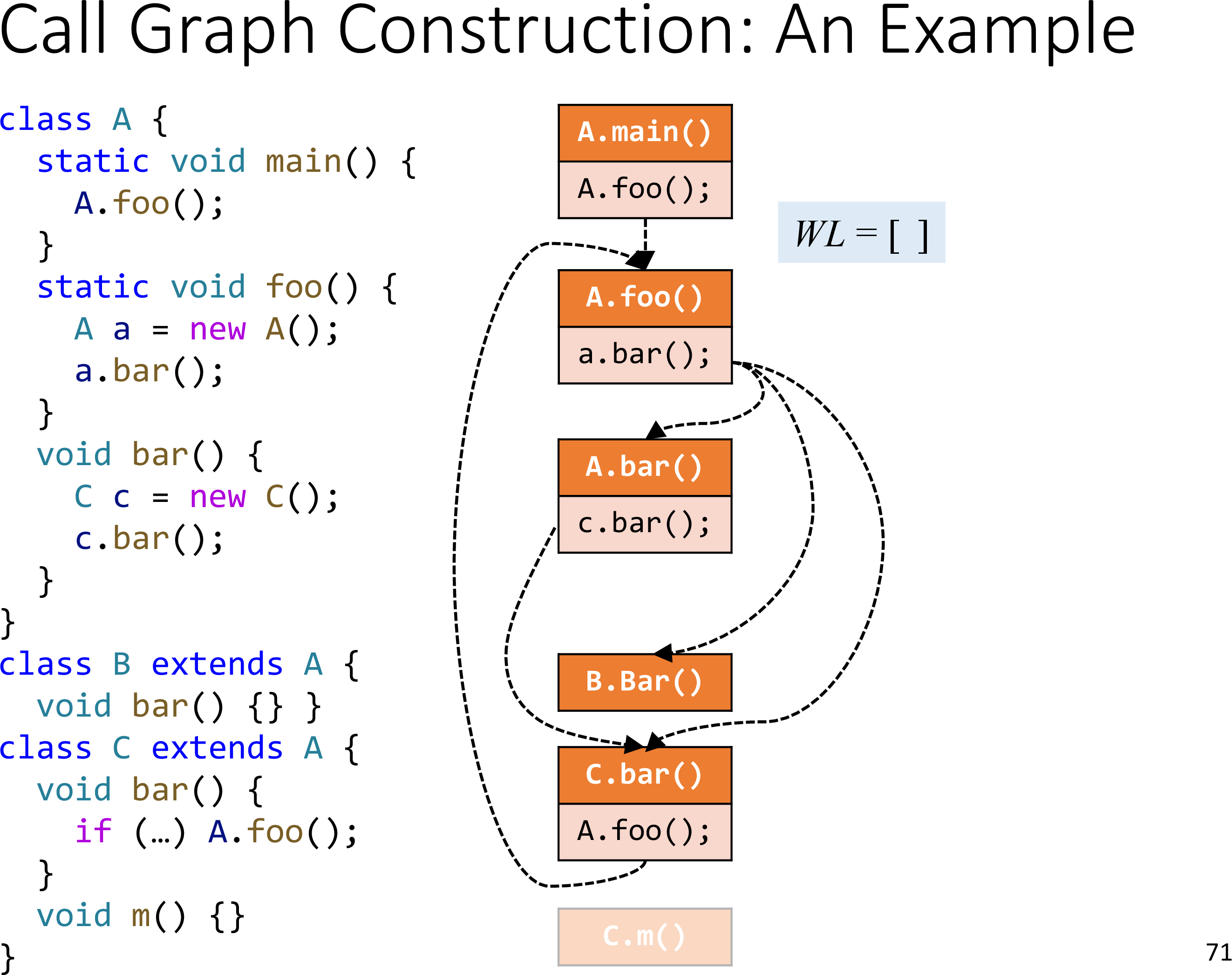
通过 Resolve 就可以构造调用图了
一个例子
Concept of interprocedural control-flow graph
相较于 control-flow graph 而言
多了调用和返回的边
ICFG = CFGs + call & return edges
Concept of interprocedural data-flow analysis
相较于 intraprocedural data-flow analysis 而言
需要考虑 call & return edges 的 transfer functions
Interprocedural constant propagation
以过程间常量传播为例
直接看一个例子
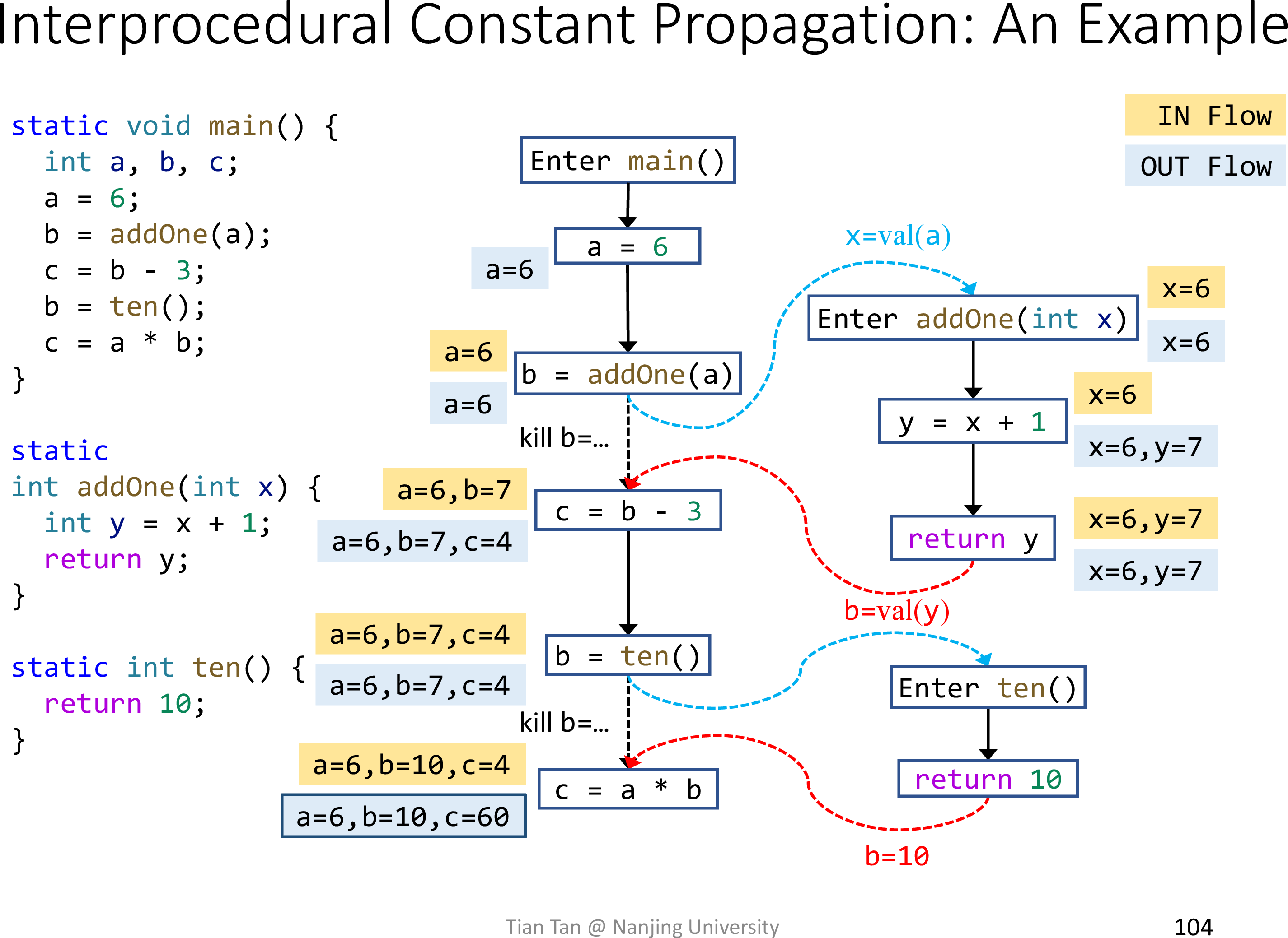
有两处细节需要注意
- 过程调用语句不仅有
call edges,也保留了原始的边,这是为了传播原作用域的常量- 例如
b = addOne(a)的 outFact 保留了a = 6 - 否则就需要在过程中传播这些常量,并且无法处理变量重名的情形
- 例如
- 过程调用语句的 transfer functions 中需要 kill LHS
- 否则就可能与
return edges中的 fact 作用产生 NAC
- 否则就可能与
可以对比原版常量传播
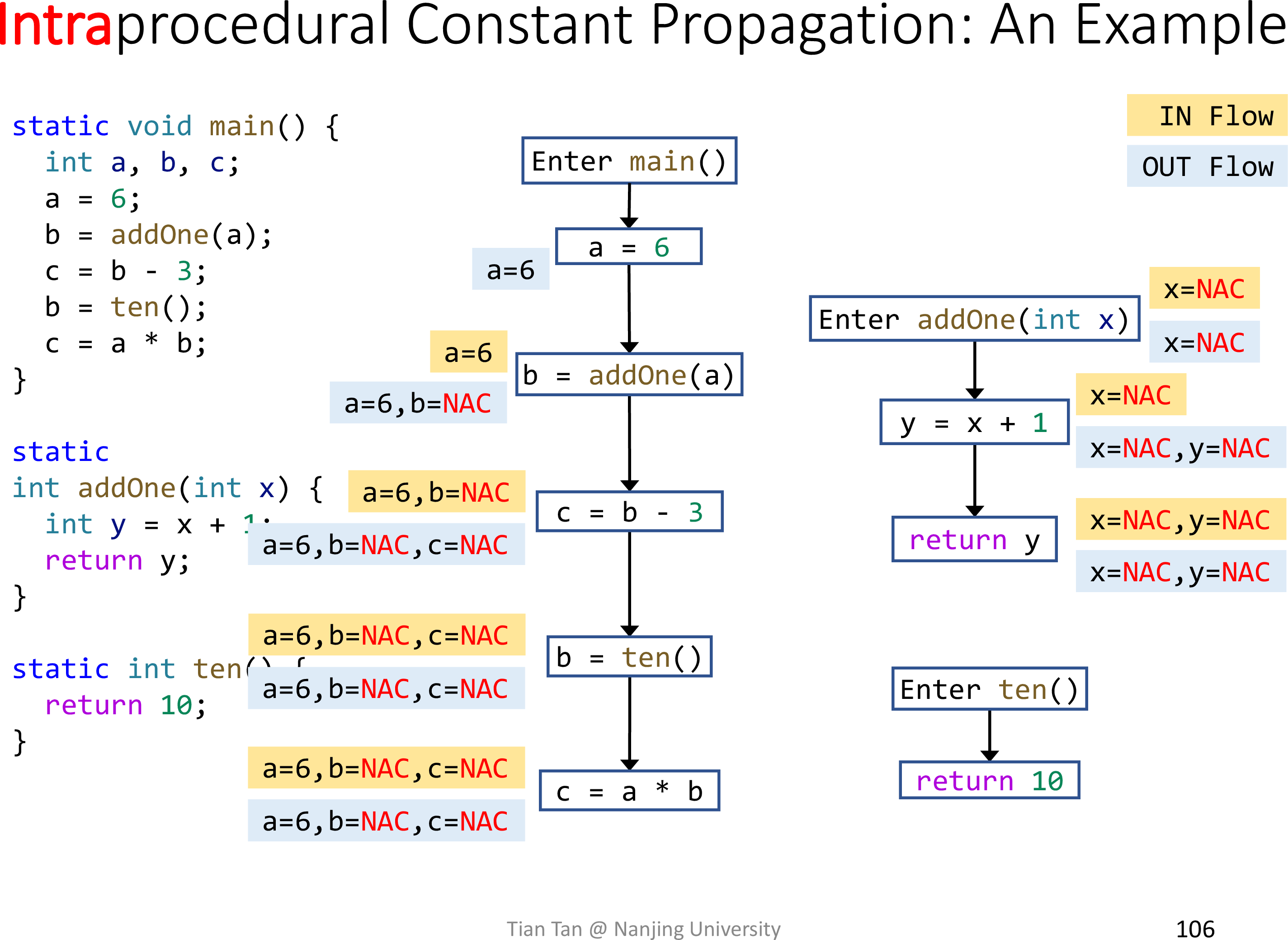
参数和返回值均为 NAC
A4
note
CHA
直接翻译课件的算法即可
完成后可以进行 CHATest
通过配置 Assignment 类的 Run Configuration 来生成 ICFG,图类似于
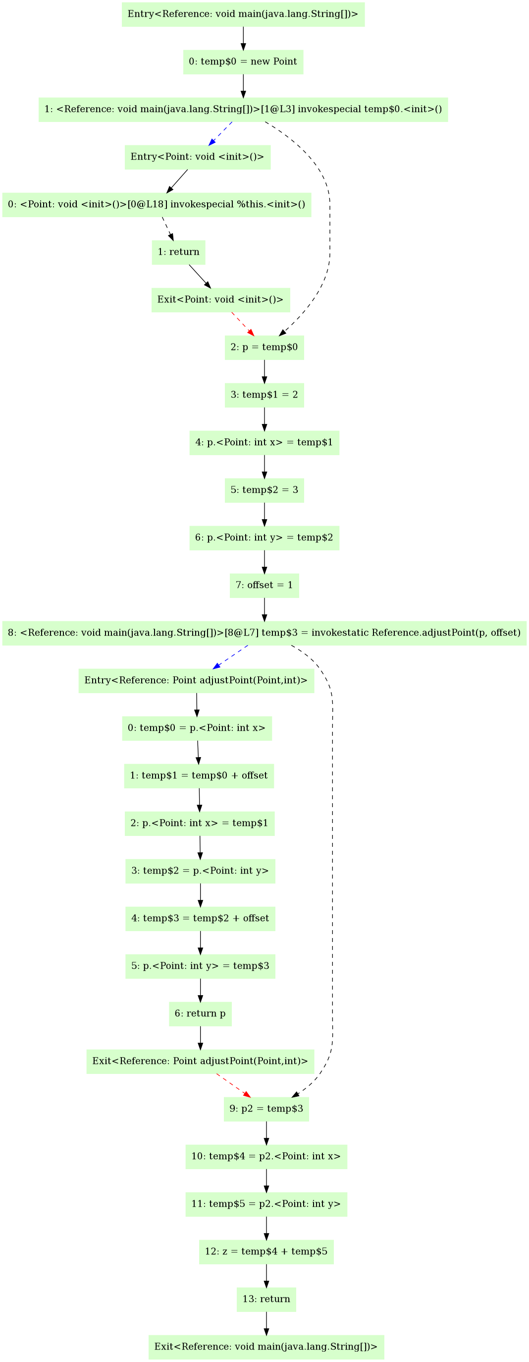
- 黑实线 - NormalEdge
- 黑虚线 - CallToReturnEdge
- 蓝虚线 - CallEdge
- 红虚线 - ReturnEdge
另外,详解一下 Invoke
- 对于一个语句
b = a.m(...)来说,b是result,a.m(...)是InvokeExp f(...) {...; b = a.m(...); ...;},在这里f(...)是b = a.m(...)的containerMethodRef信息保存在InvokeExp中
interprocedural constant propagation
主要实现结点和边的 Transfer function
AbstractInterDataflowAnalysis 类会会根据结点和边的类型,在 transferEdge 和 transferNode 函数内部调用这些 Transfer function
参考课件
Node transfer
- Call nodes: identity
- Other nodes: same as intraprocedural constant propagation
Edge transfer
-
Normal edges: identity
-
Call-to-return edges: kill the value of LHS variable of the call site, propagate values of other local variables
-
Call edges: pass argument values
-
Return edges: pass return values
不要忘了 Java 的对象管理机制
- 不要修改
outFact - 也不要在 identity func 中直接返回
outFact
interprocedural worklist solver
类似 intraprocedural worklist solver
有两处变动
- 仅对 entryMethod 的 entryNode 初始化
newBoundaryFact,其余均为newInitialFact - IN 的修改方法,从遍历
cfg.predsOf变成了遍历icfg.inEdgesOf,其中施以transferEdge
submit
压缩命令
zip -j 201250012.zip src/main/java/pascal/taie/analysis/dataflow/inter/InterSolver.java src/main/java/pascal/taie/analysis/dataflow/inter/InterConstantPropagation.java src/main/java/pascal/taie/analysis/graph/callgraph/CHABuilder.java- 参考
Reference.java本地测试用例,考虑如下两个 stmttemp$0 = new Point,右侧 exp 为 NewExp,应为 UNDEFtemp$0 = p.<Point: int x>,右侧 exp 为 FieldAccess,若其 FieldRef 的类型 canHoldInt,应为 NAC
- 于是增补
evaluate函数,A2 多通过了 3 个用例 - 2 个 interprocedural constant propagation 的测试用例未通过
- 发现对于 kill LHS 的处理有误,不应该在
transferCallNode中处理,而应在transferCallToReturnEdge中处理 - 很好奇有什么区别……
PTA
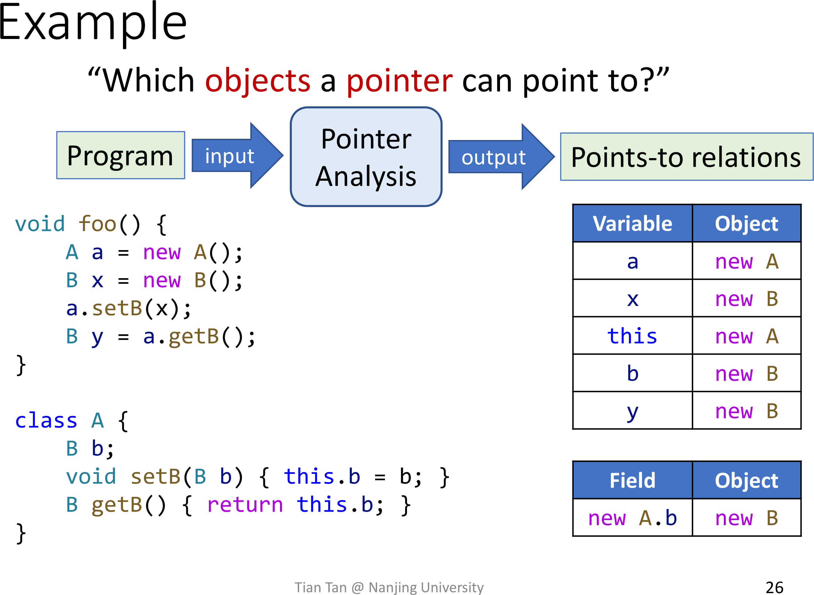
What is pointer analysis?
Which objects a pointer can point to?
Understand the key factors of pointer analysis
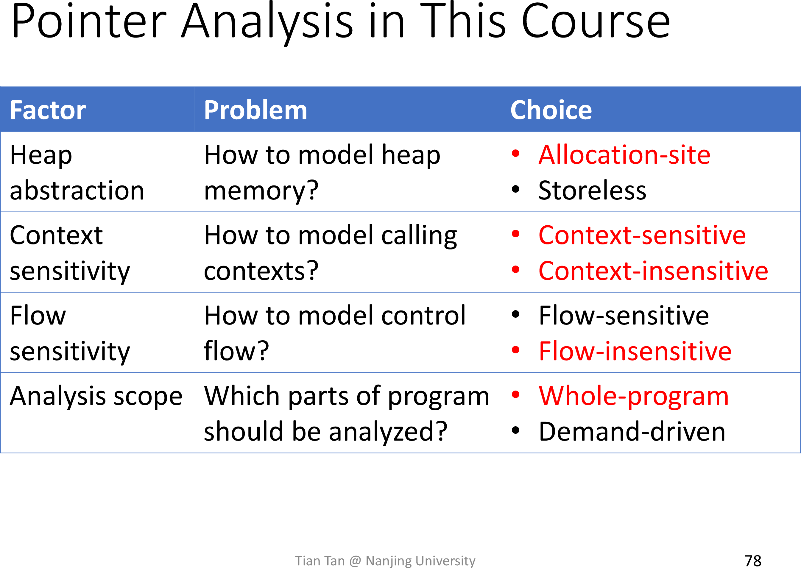
- Heap Abstraction - How to model heap memory?
- 在循环中可能创建无限的对象
- 考虑在 allocation site 处建模对象,因为 allocation site 是有限的
- Context Sensitivity - How to model calling contexts?
- 对于同一个方法,在不同的调用上下文下是否需要重新分析
- Flow Sensitivity - How to model control flow?
- 是否考虑语句的执行顺序
- Analysis Scope - Which parts of program should be analyzed?
- 直接全程序分析
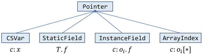
Understand what we analyze in pointer analysis
pointers in Java
- Local variable:
x - Static field:
C.f - Instance field:
x.f - Array element:
array[i]
对于数组而言,不考虑下标
pointer-affecting statements
| type | example |
|---|---|
| New | x = new T() |
| Assign | x = y |
| Store | x.f = y |
| Load | y = x.f |
| Call | r = x.k(a, …) |
对于方法调用而言,考虑最复杂的 Virtual call
PTA-FD
Understand pointer analysis rules
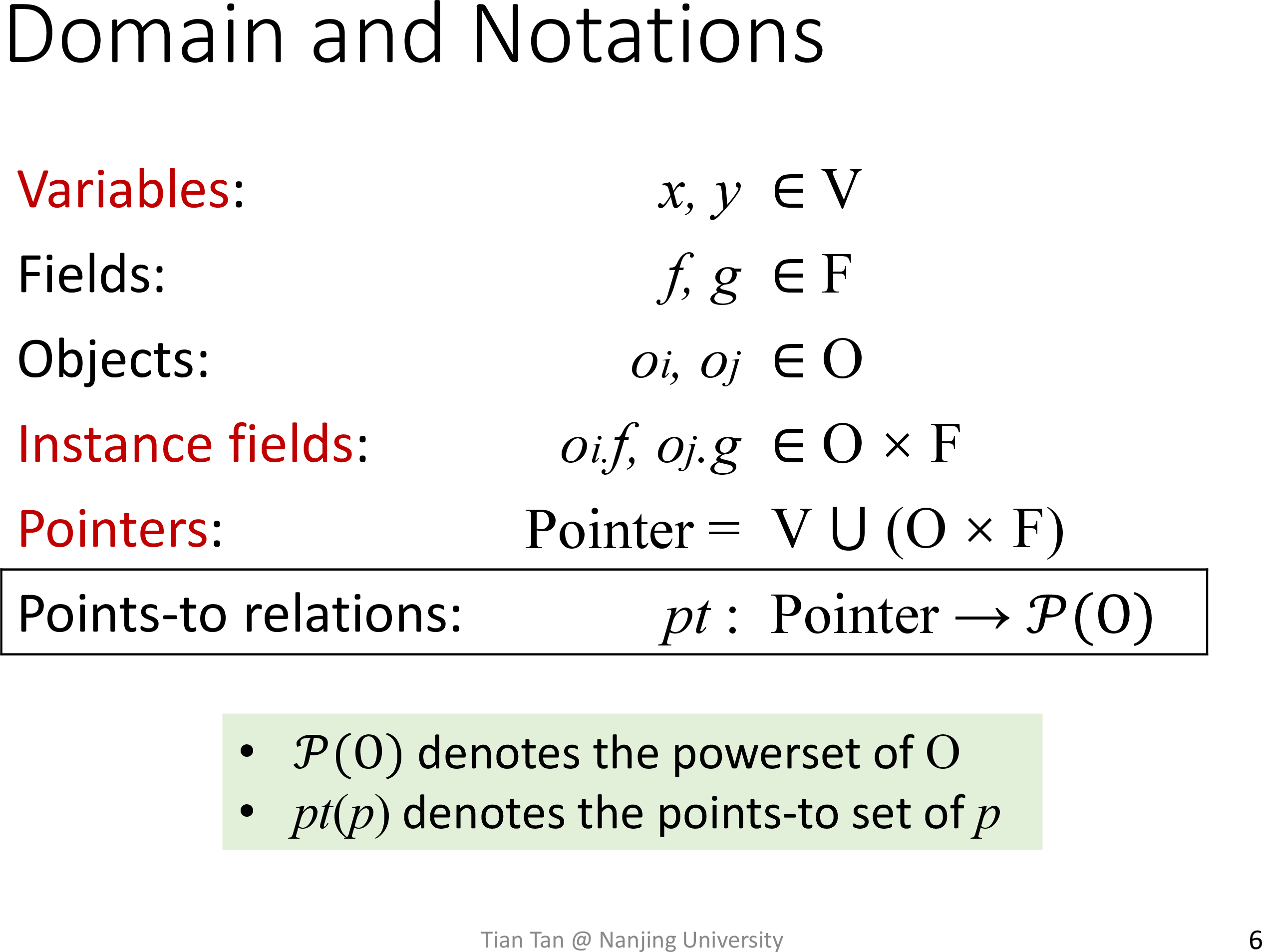
先约定一些记号
不考虑函数调用,有如下规则
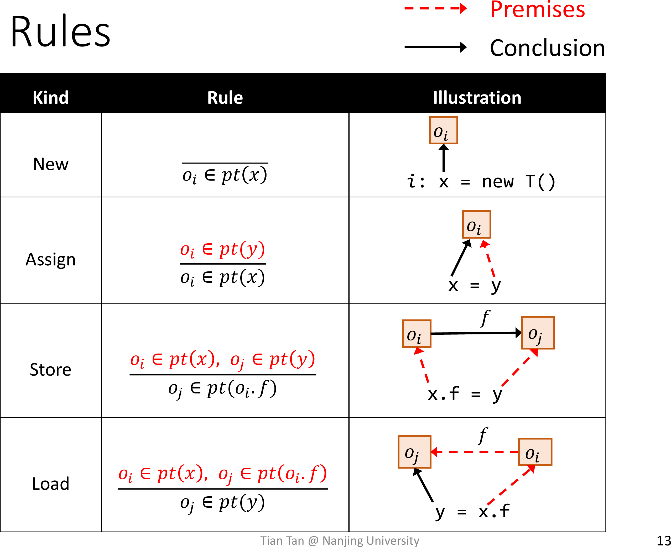
Understand pointer flow graph
With PFG, pointer analysis can be solved by computing transitive closure of the PFG
PFG is dynamically updated during pointer analysis
- 顶点
Pointer = V ⋃ (O × F)
- 边
An edge 𝑥 → 𝑦 means that the objects pointed by pointer 𝑥 may flow to (and also be pointed to by) pointer 𝑦
Understand pointer analysis algorithms
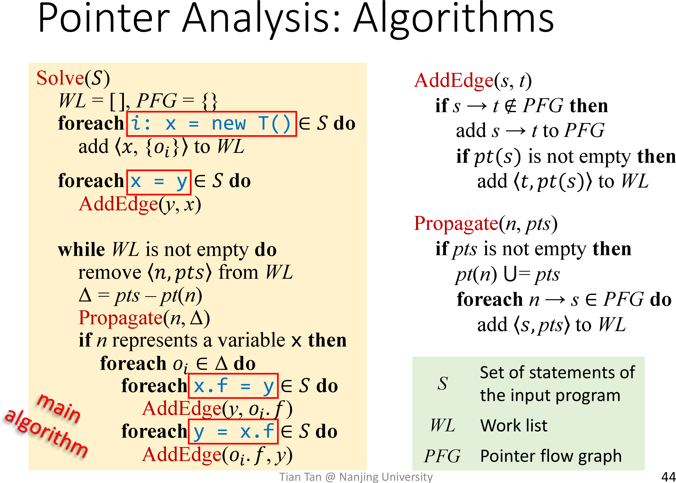
关注 Propagate 前需要去重
判断 n represents a variable x,也就是判断 n 作为 Pointer 是 V 而非 O × F
对于链式调用,JVM 会进行分解
Understand pointer analysis rule for method call
实际上从 intra 扩展为 inter
考虑函数调用的规则
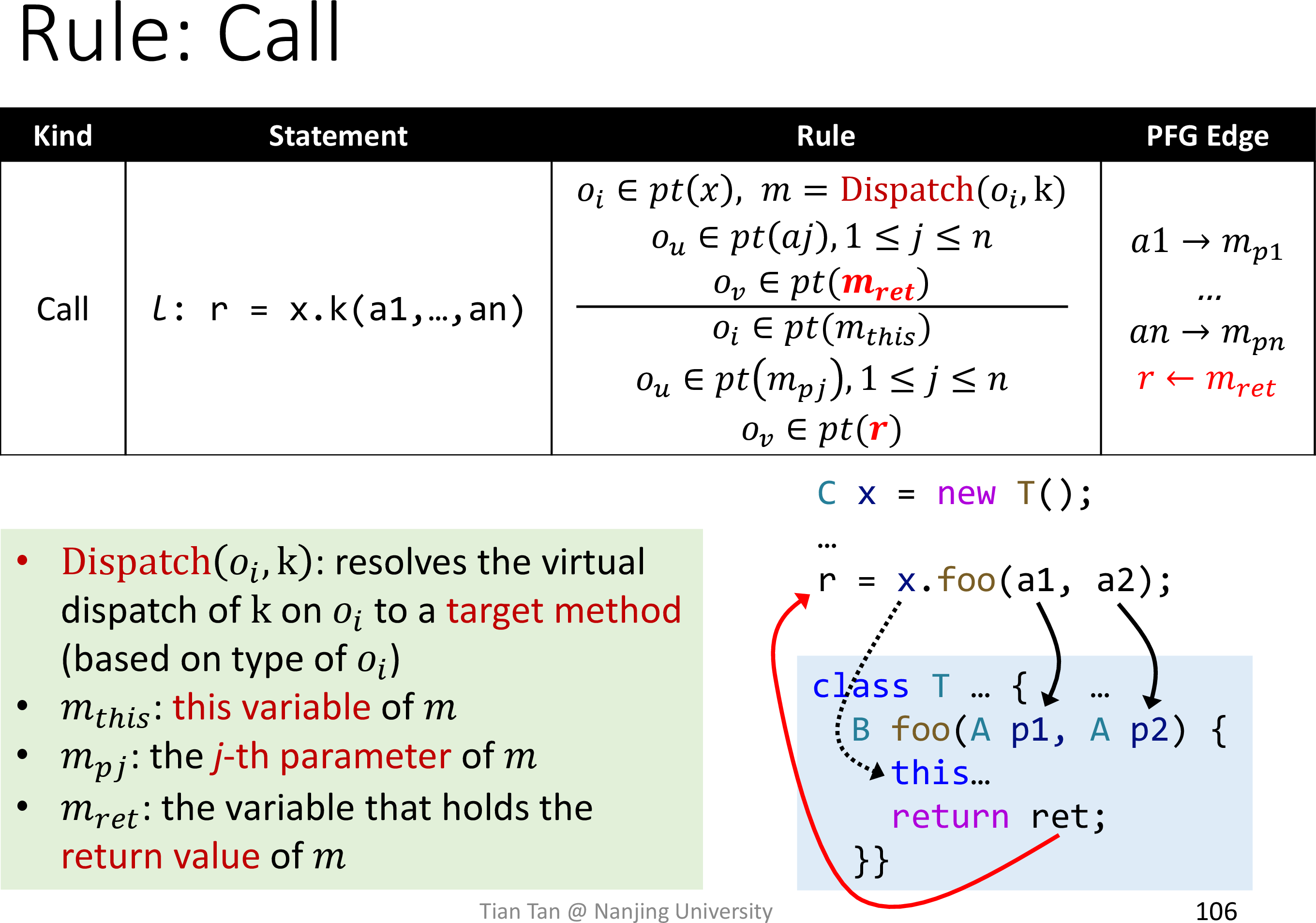
四步走
- 解析方法
- 传递 this - 不需要添加边,因为 this 指针指向的对象是确定的
- 传递参数 - 在 PFG 中添加边
- 传递返回值 - 在 PFG 中添加边
Understand inter-procedural pointer analysis algorithm
更新算法
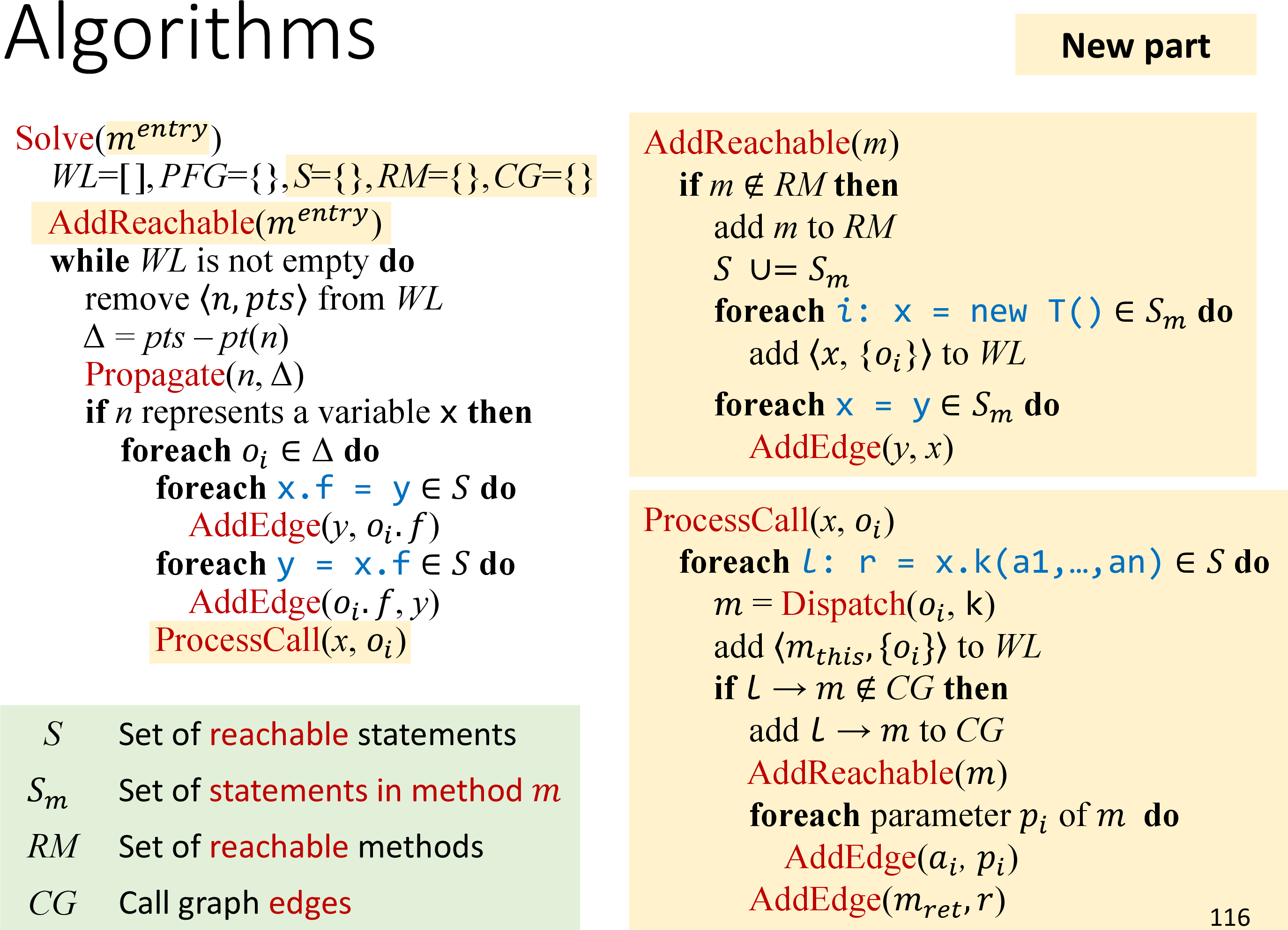
在 AddReachable 中统一处理 New 和 Assign
Understand on-the-fly call graph construction
注意到在算法进行的过程中构建了调用图
类似之前 pointer flow graph 的动态更新
也就是算法的最终产物有两个
- Pointer analysis
- Call graph
A5
note
关注的 pointer-affecting statements 如下
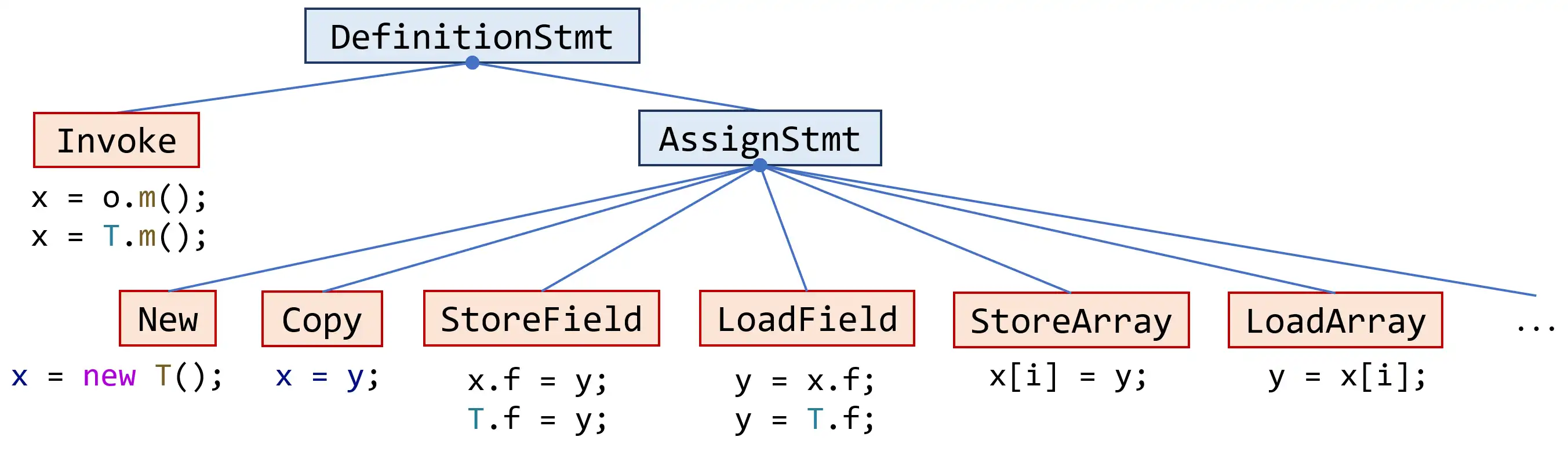
注意 Invoke / StoreField / LoadField 中存在静态调用或字段
对于实现了访问者模式的 StmtProcessor 类,只需要处理 statements in new reachable methods 即可,也就是如下 stmt
- New
- Copy
- Invoke (static)
- StoreField (static)
- LoadField (static)
而 analyze 中需要处理如下 stmt
- Invoke -
processCall - StoreField
- LoadField
- StoreArray
- LoadArray
静态方法的解析可以使用
invoke.getMethodRef().resolve();非静态方法的解析使用
resolveCallee(recv, invoke);注意区分 callGraph 和 pointerFlowGraph
在 addPFGEdge 时填充 workList
在 propagate 中填充每个 pointer 的 pointsToSet
对于 StoreArray 和 LoadArray 而言,pointer 就是 obj,并没有使用 stmt 自身
对于算法中的 Set of reachable statements,由于 Var 类中提供了 RelevantStmts,就不必记录了
submit
压缩命令
zip -j 201250012.zip src/main/java/pascal/taie/analysis/pta/ci/Solver.javaPTA-CS
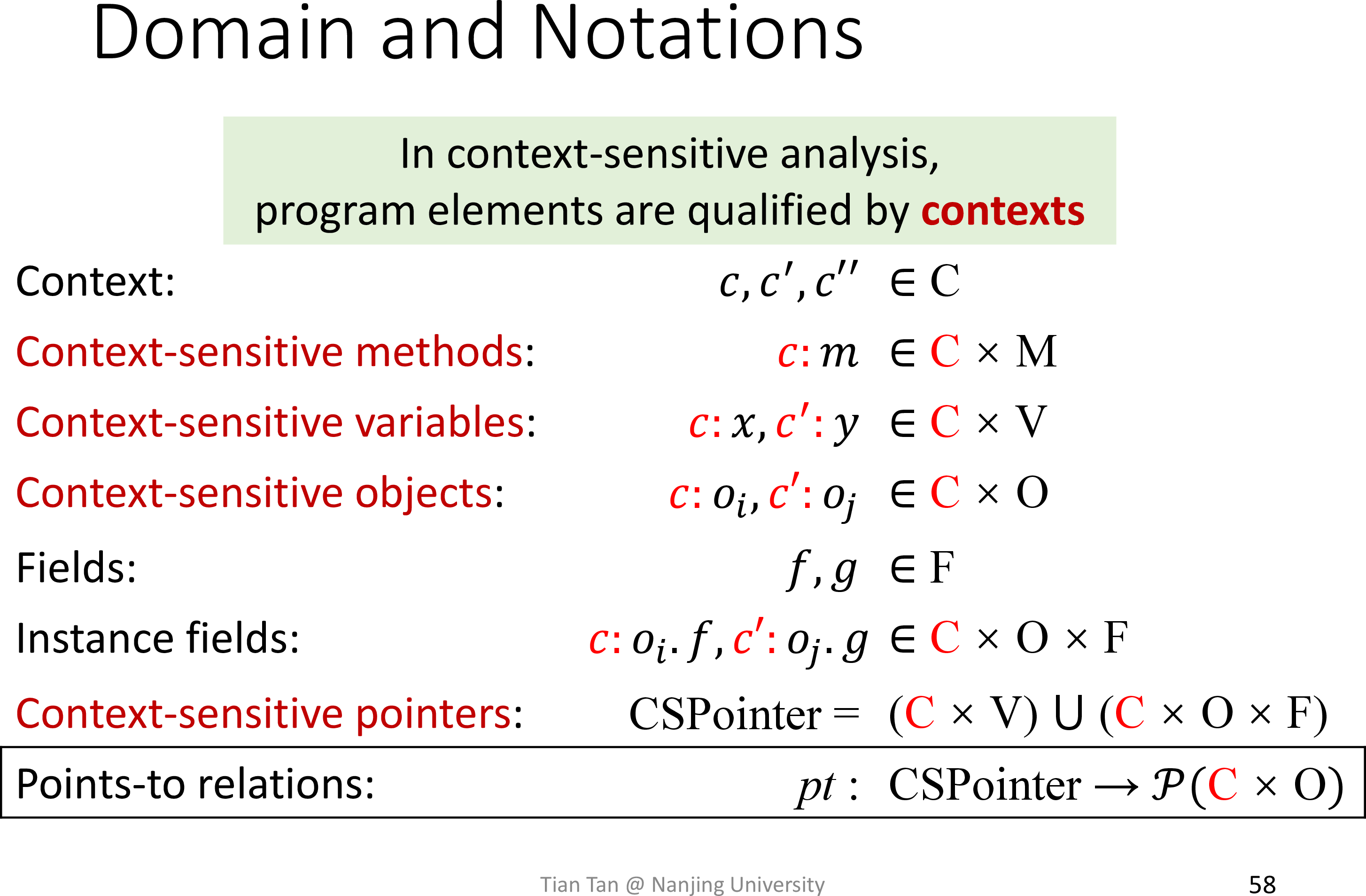
Concept of context sensitivity (C.S.)
method 和 variable 持有上下文
单独分析不同的上下文
Cloning-Based Context Sensitivity
Concept of context-sensitive heap (C.S. heap)
object 也持有上下文
Why C.S. and C.S. heap improve precision
一个例子
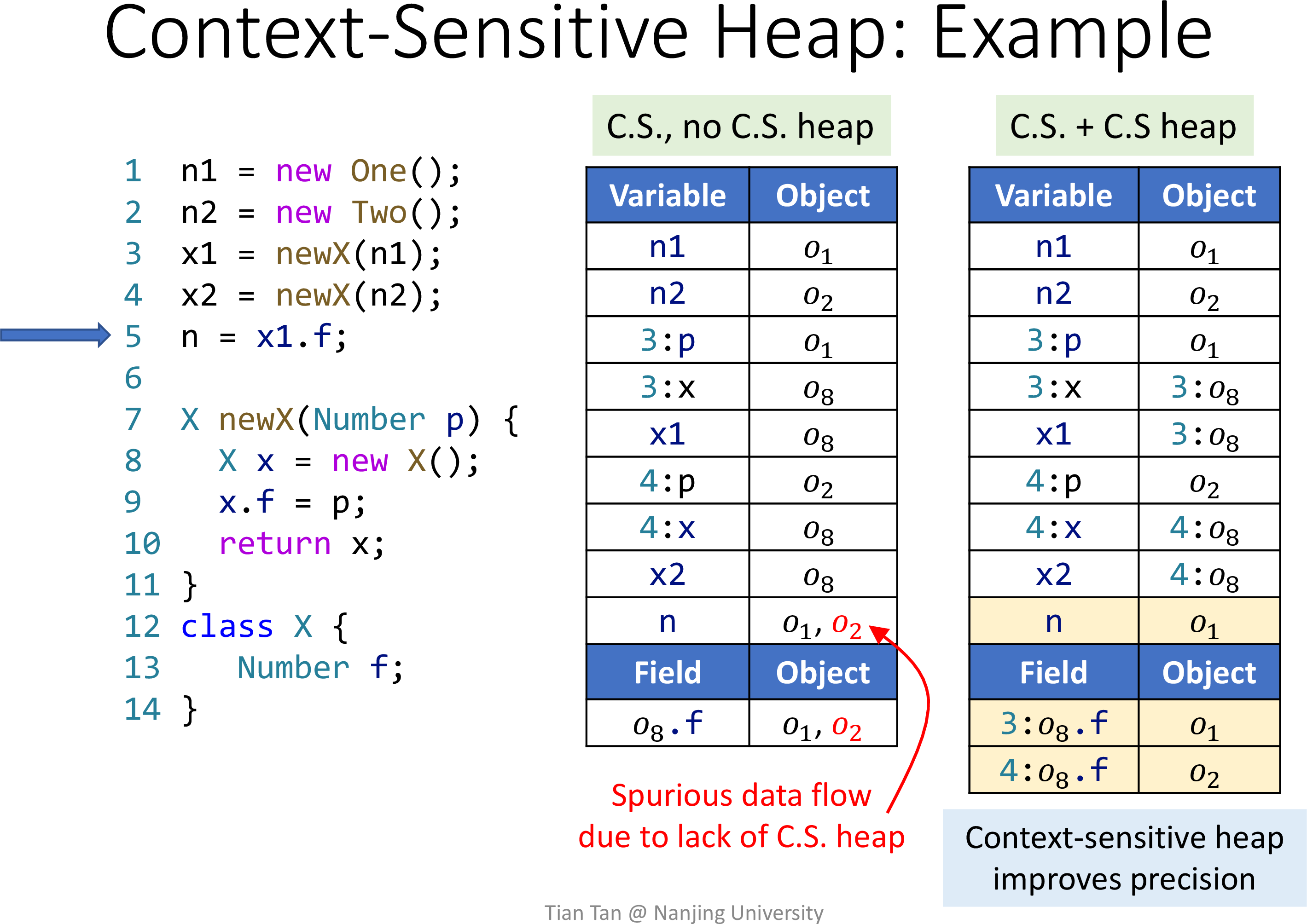
这里的上下文为 callsite
本质上是在一个方法中传递的参数影响了 New 生成的对象
Without C.S., C.S. heap cannot improve precision
Context-sensitive pointer analysis rules
约定一些记号
使用 C.S. + C.S heap
其规则类似 C.I.,多了一些上下文
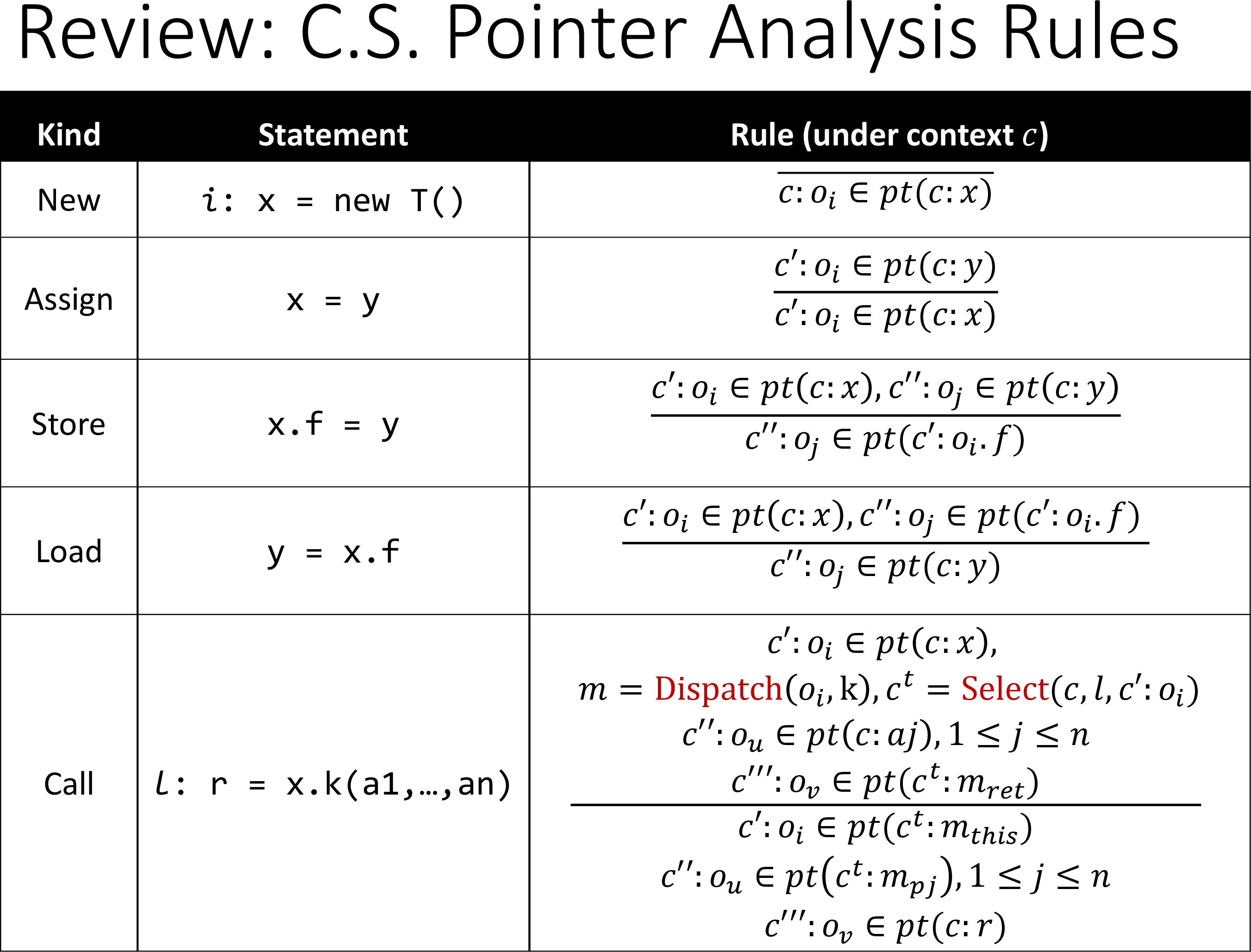
在 Call 中添加了 Select,考虑如下因素
- caller context -
- callsite
- receiver object with heap context
注意 callee 的 context 为
Algorithm for context-sensitive pointer analysis
算法与 C.I. 几乎完全一致
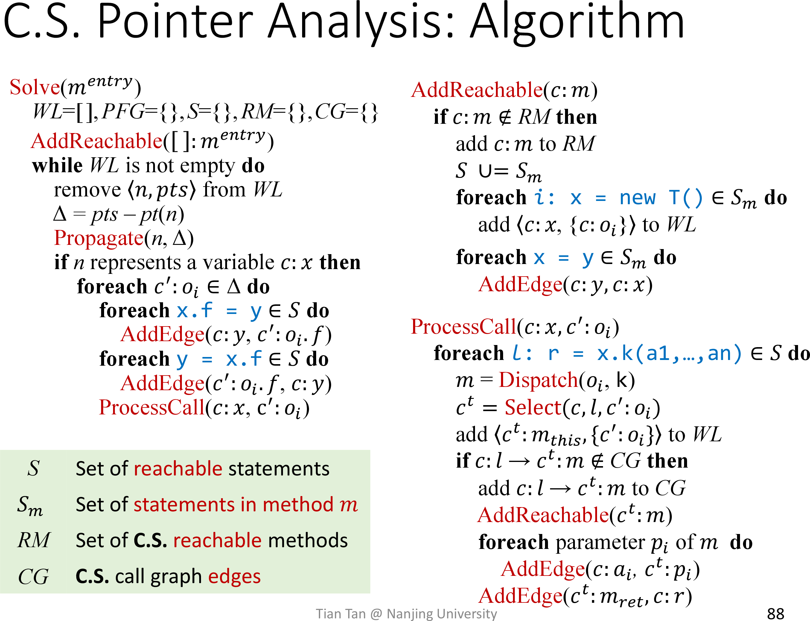
注意 entry 的上下文为空
所有新的上下文均通过 Select 生成
Common context sensitivity variants
Call-site sensitivity
call-string sensitivity, or k-CFA
Select(c, l, _) = [l1, ..., ln, l] where c = [l1, ..., ln]类似调用栈中的行号链
一个例子
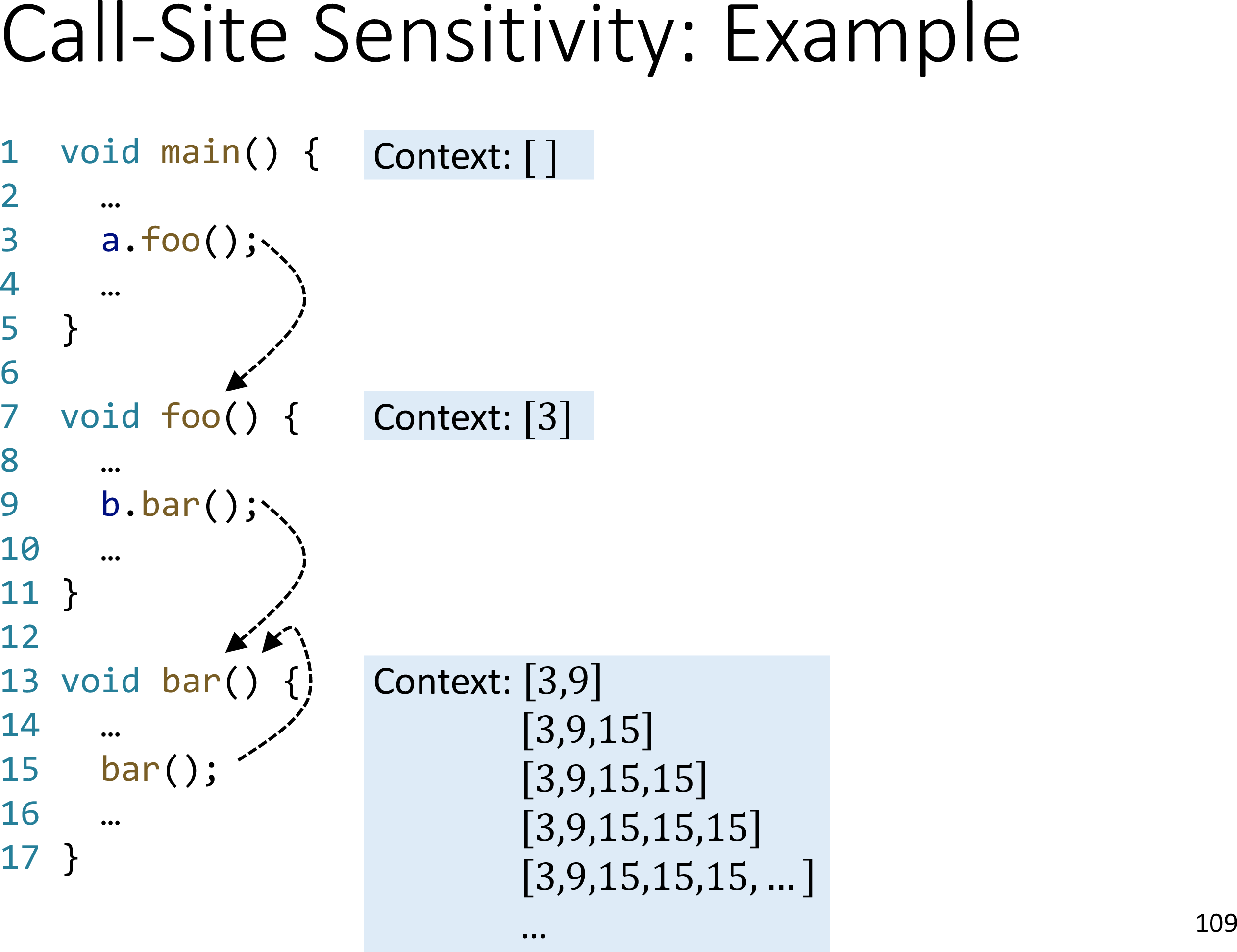
注意到递归调用可能产生无限的 context
于是限制 context 的大小
显然对于 1-call-site / 1-CFA 而言
Select(_, l, _) = [l]Object sensitivity
Select(_, _, c':O) = [O1, ..., On, O] where c' = [O1, ..., On]Type sensitivity
coarser abstraction over object sensitivity
Select(_, _, c':O) = [t1, ..., tn, InType(O)] where c' = [t1, ..., tn]InType 定义如下
class X { void m() { Y y = new Y(); }}则 InType(O3) = X
Differences and relationship among common context sensitivity variants
一个例子来对比三种 context sensitivity
class X {    void main() {        Y y1 = new Y();        y1.foo();        y1.foo();        Y y2 = new Y();        y2.foo();    }}
class Y {    void foo() {}}
Contexts of foo()
- Call-site sensitivity
[4, 5, 7]- Object-sensitivity
[O3, O6]- Type-sensitivity
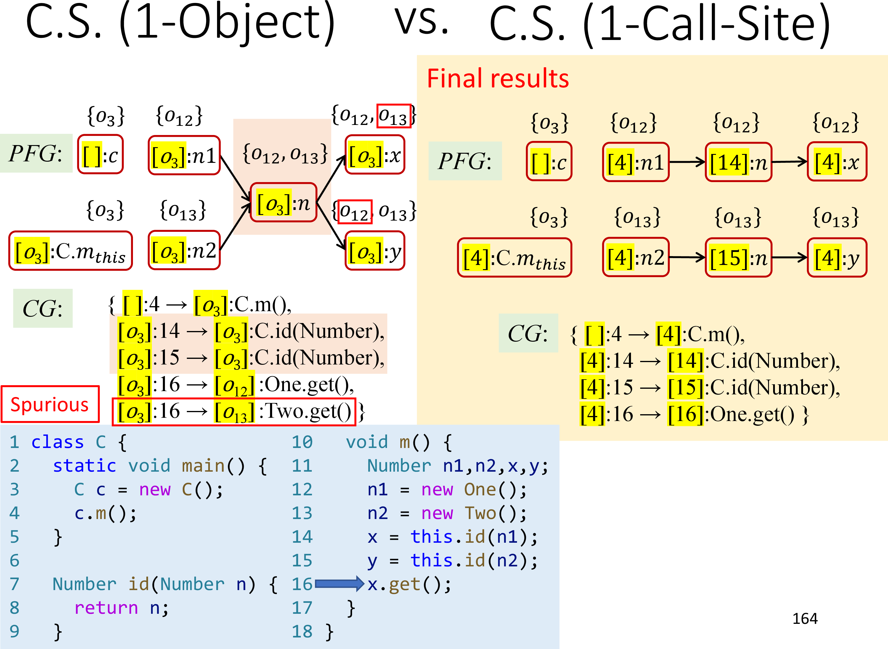
[X]Call-Site vs. Object Sensitivity
不同的场景下有不同的结果
For simplicity, we do not apply
C.S. heapand omit this variable
场景一

Call-Site Sensitivity 产生 Spurious 结果的原因如下
- 同一条 Call 语句的上下文不同
- 而
1-CFA的上下文只考虑调用时的行号,无法进行区分
场景二
Object Sensitivity 产生 Spurious 结果的原因如下
1-Object的上下文只考虑调用的 receiver object- 若使用相同的 receiver object 调用但参数不同,则无法区分
一般的,对 OO 而言
- Precision: object > type > call-site
- Efficiency: type > object > call-site
A6
note
Solver
对于 C.S. 而言,Pointer 是有上下文的
于是引入 CSElement 接口
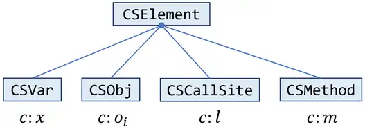
这里的 CSCallSite 实际上合并了算法中 Select 函数的前两个参数
只要在有上下文的 Pointer 中包含上下文信息即可
在 A5 中使用 PointerFlowGraph 类来管理无上下文的 Pointer
A6 则单独引入了 CSManager 类来管理有上下文的 Pointer
另外引入了 PointsToSetFactory 工厂类,通过 CSObj 构造 PointsToSet
注意 New 语句中上下文的处理
要根据 Container Method 得到 HeapContext
Context objContext = contextSelector.selectHeapContext(csMethod, null); // noteworkList.addEntry( csManager.getCSVar(context, stmt.getLValue()), PointsToSetFactory.make( csManager.getCSObj(objContext, heapModel.getObj(stmt))));注意 Call 语句中上下文的处理
- 对于静态方法而言
根据 CSCallSite 得到 calleeContext
CSCallSite callSite = csManager.getCSCallSite(context, stmt);Context calleeContext = contextSelector.selectContext(callSite, null);callerContext 即为 Container Method 的 Context
- 对于非静态方法而言
根据 CSCallSite 和 CSObj 得到 calleeContext
CSCallSite callSite = csManager.getCSCallSite(recv.getContext(), invoke);Context calleeContext = contextSelector.selectContext(callSite, recvObj, null);callerContext 即为 CSVar 的上下文
objContext 即为 CSObj 的上下文
Selector
先考虑 selectHeapContext
约定 k 层的 context selector,其 heap context 的层数为 k - 1,于是
- 对于 1-limiting 的 Selector
return getEmptyContext();- 对于 2-limiting 的 Selector
switch (method.getContext().getLength()) { case 0: return getEmptyContext(); case 1: return ListContext.make(method.getContext().getElementAt(0)); case 2: return ListContext.make(method.getContext().getElementAt(1)); default: assert false;}return null;再考虑 selectContext
- 对于
CallSelector而言,静态和非静态的处理是一致的,只需要关注CSCallSite即可 - 对于
ObjSelector和TypeSelector而言,静态直接返回调用者方法的上下文,而非静态只需要关注CSObj
注意不要混淆
CSCallSite和CSObj的上下文
submit
压缩命令
zip -j 201250012.zip src/main/java/pascal/taie/analysis/pta/cs/Solver.java src/main/java/pascal/taie/analysis/pta/core/cs/selector/_*.javaA7
note
参考 StaticFieldMultiStores.java 本地测试用例
- 发现 A6 中静态方法调用忘记修改调用图了……
- 因为 A6 仅检查指针分析的结果,所以并没有检测出来……
仅修改 transferNonCallNode 一个函数,思路如下
- 对于
StoreXXX,将所有对应的LoadXXX加入 workList,然后直接调用(intra) transferNode - 对于
LoadXXX,根据所有对应StoreXXX得到对应的 value 并进行 meet,不用调用(intra)transferNode - 注意到 A2 的
(intra) transferNode不考虑 LHS 为 FieldAccess 或 ArrayAccess 等复杂情形(尽管需要进行正确的处理)
关于对应,根据实验指南总结如下
- 实例字段
- base(Var) 对应的 PointsToSet 有交集
- field 一致
- 静态字段
- class 一致
- field 一致
- 不需要指针分析的结果
- 数组
- base(Var) 对应的 PointsToSet 有交集
- index(Var) 满足一定的要求
关于从对应 StoreXXX 得到对应的 value,需要获取 StoreXXX 的 outFact
- 例如
o.f = x然后y = o.f,只有分析了StoreXXX,才能从 outFact 得到x = ... - 由于数组的 index 也是 Var,所以在处理数组的
StoreXXX和LoadXXX时,需要同时获取StoreXXX和LoadXXX的 outFact - 参考
ArrayInter2.java本地测试用例,发现也需要关注传入的参数 inFact,因为其中也可能包含 index 的 Value
在具体实现上
- 由于 InterConstantPropagation 类中拥有 InterSolver 类的实例
- 而只有在 InterSolver 类才能修改 workList,并获取 DataflowResult 得到各种 fact 信息
- 为此 InterSolver 类增加 2 个 API
public DataflowResult<Node, Fact> getResult() {    return result;}
public void addWorkList(Node node) { workList.add(node);}transferNonCallNode对不同 stmt 的处理可以使用访问者模式实现- 并未考虑 FieldAccess 或 ArrayAccess 具体的 Type 信息,例如 canHoldInt
submit
压缩命令
zip -j 201250012.zip src/main/java/pascal/taie/analysis/dataflow/inter/InterSolver.java src/main/java/pascal/taie/analysis/dataflow/inter/InterConstantPropagation.java src/main/java/pascal/taie/analysis/dataflow/analysis/constprop/ConstantPropagation.javaSecurity
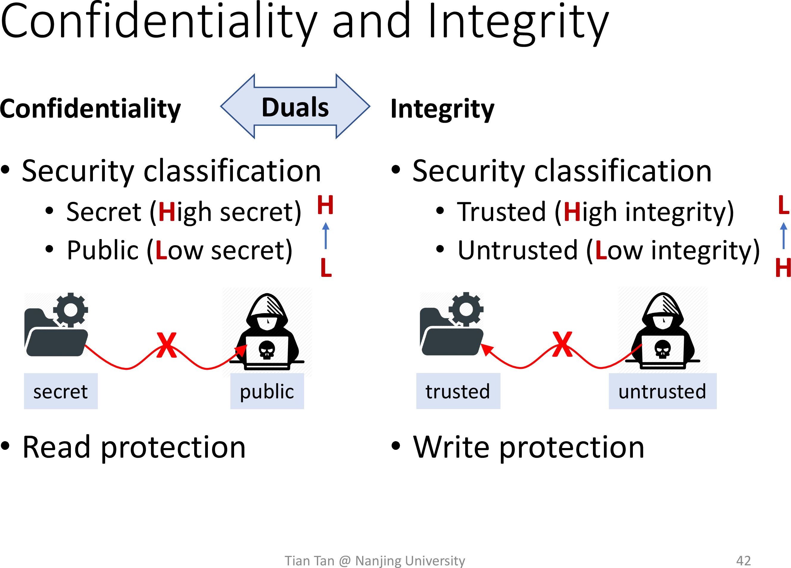
Concept of information flow security
- Classifies program variables into different security levels
- Specifies permissible flows between these levels, i.e., information flow policy
- The most basic model is two-level policy, i.e., a variable is classified into one of two security levels
- H, meaning high security, secret information
- L, meaning low security, public observable information
- Requires the information of high variables have no effecton (i.e., should not interfere with) the information of low variables
- - ×
- - √
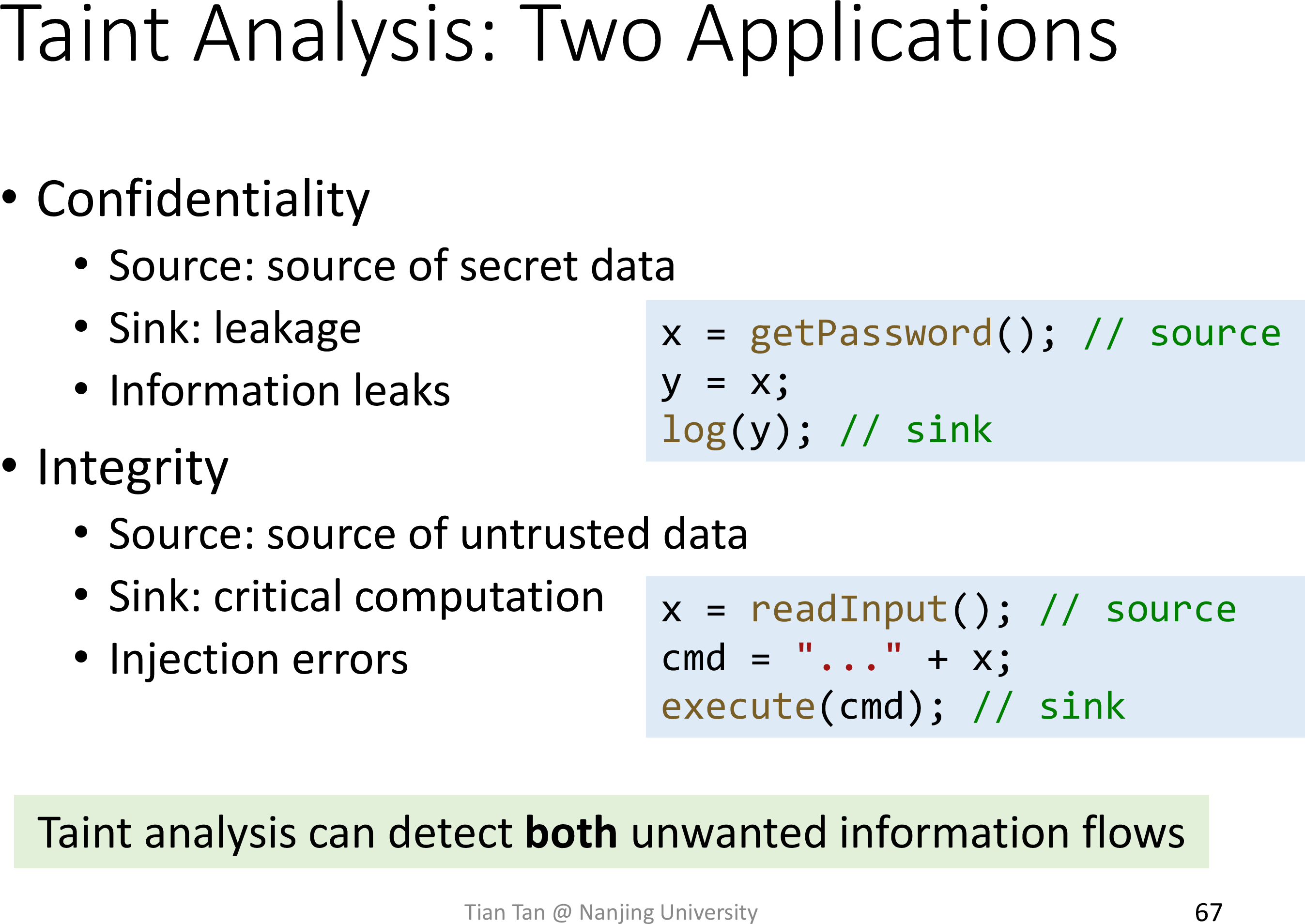
Confidentiality and integrity
- Confidentiality - Prevent secret information from being leaked
- Integrity - Prevent untrusted information from corrupting (trusted) critical information
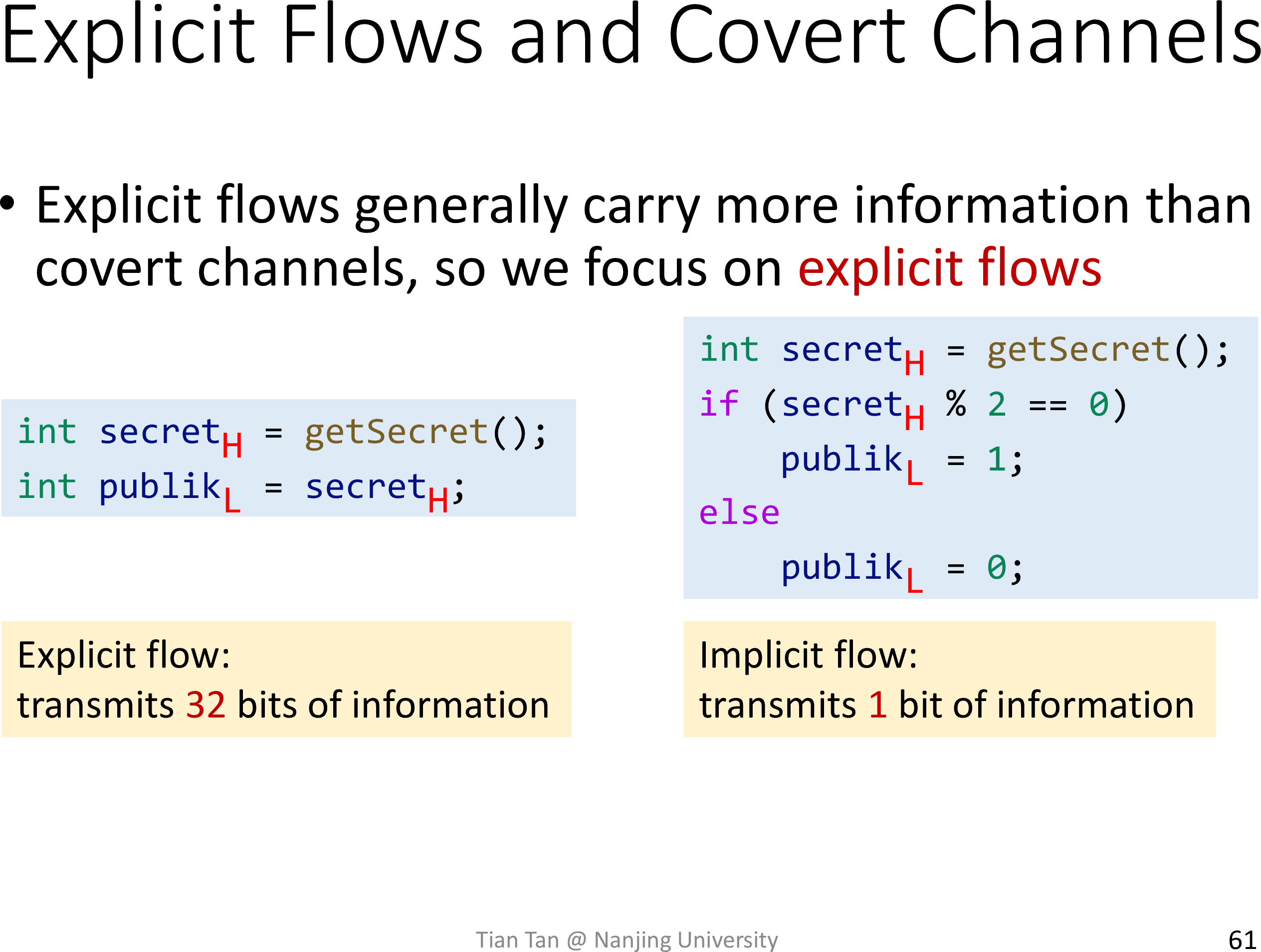
Explicit flows and covert channels
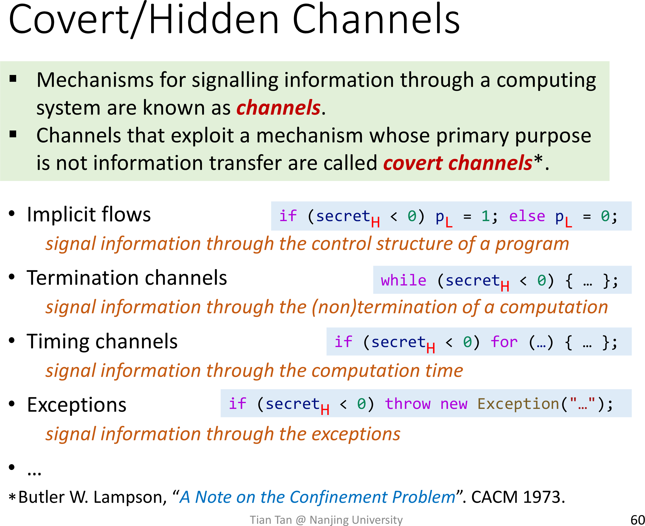
Covert/Hidden Channels
Use taint analysis to detect unwanted information flow
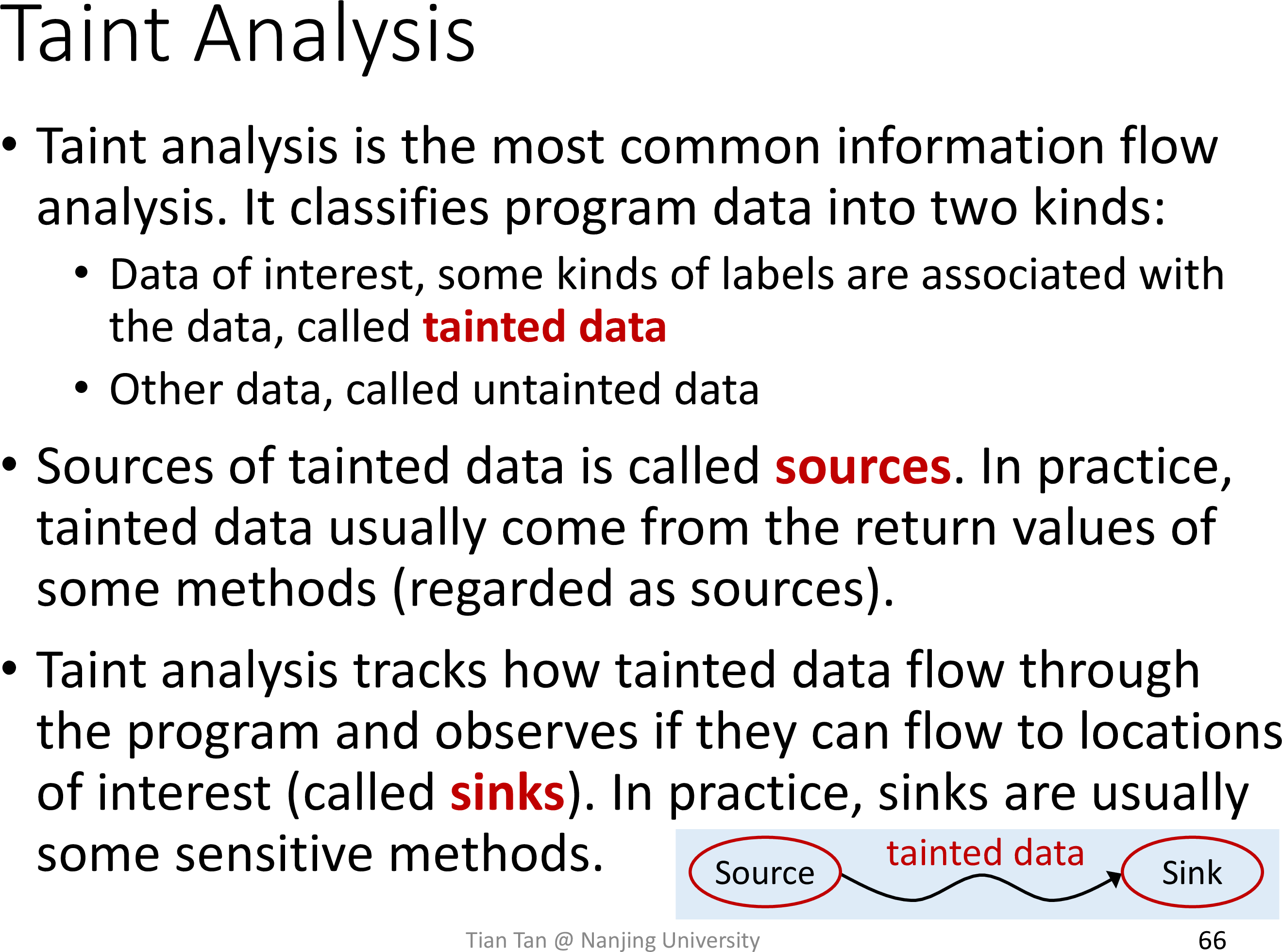
通过定义不同的 source 和 sink,就可以分析 confidentiality 和 integrity
为了使用指针分析技术来进行污点分析,简化问题为
- 非上下文敏感
- 视程序中的一部分 objects 为 tainted data
- 将 source 定义为返回 tainted data 的方法
- 将 sink 定义为若 tainted data 流入其某些参数则违反 information flow security 的方法
为此,只需添加处理 Call 语句的规则即可
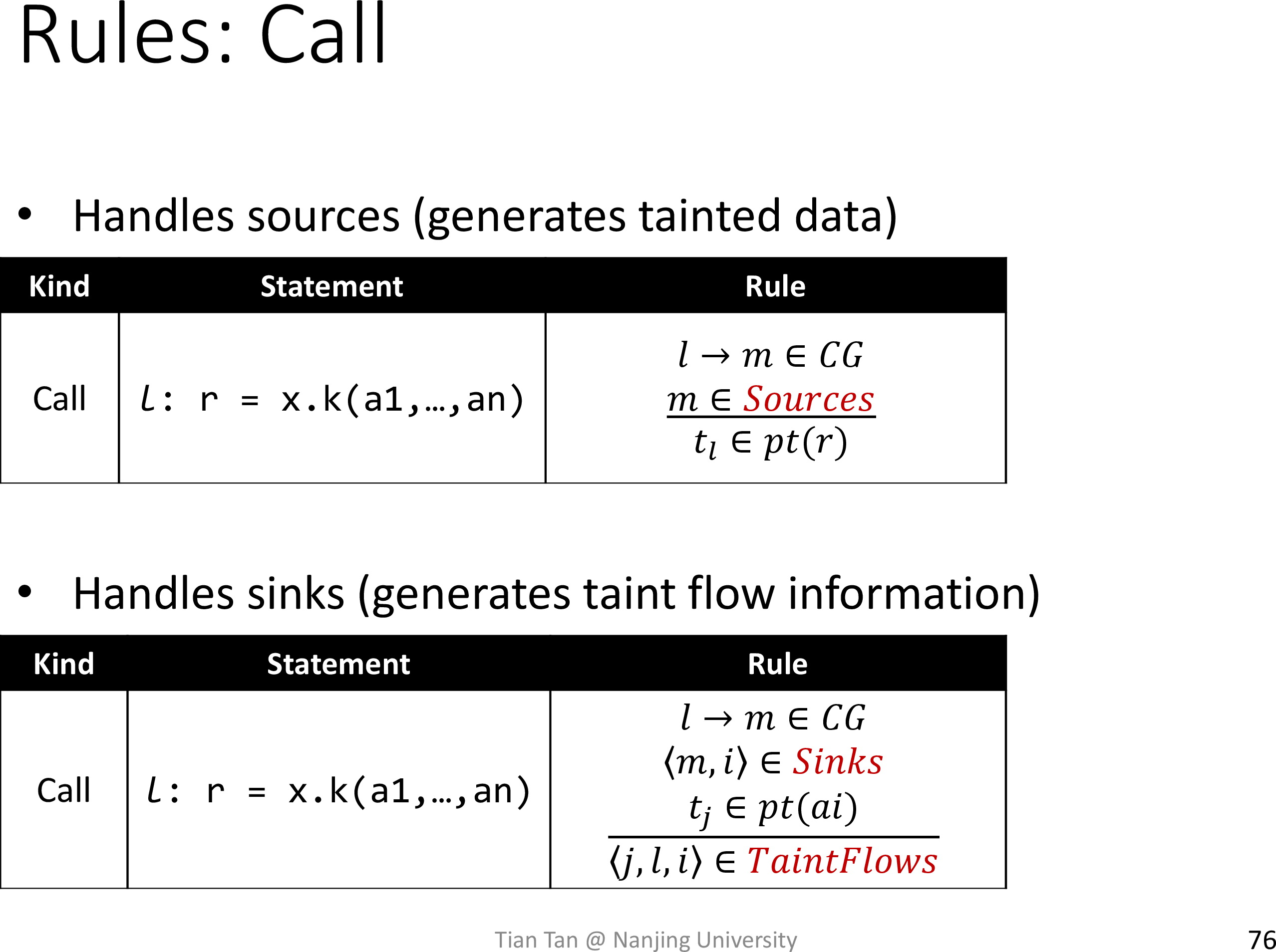
其余的规则完全不变
A8
note
本地测试用例高度依赖 jdk 版本
17.0.2 - Linux/x64
修改处理调用语句的部分,考虑如下四种情况
- process source
- process arg-to-result
- process base-to-result (non-static invoke)
- process arg-to-base (non-static invoke)
这四个函数由 TaintAnalysiss 类提供,其范式如下
- 匹配 method 和 type
对于前三种情形,type 即为 method 的 return type
而对于最后一种情形,考虑到 base pointer 可能指向其子类型的对象,所以要遍历其 PointsToSet 来提供不同的 type
- 创建 taint object
processSource 直接根据 invoke 和 return type 创建即可
其余三种情形则遍历其 PointsToSet 获取 taint object
存疑 - 是否需要匹配 taint object 的类型
若进行匹配,则类似上文,需要考虑 arg 和 base pointer 的不同类型,复杂度大增
不进行匹配似乎也没有出现 false positives
然后改变其 return type 创建新的 taint object 即可
- 加入 work list
非常 tricky 的一个地方
注意到在指针分析的处理框架中,taint object 是加入 work list 和其余对象一同被处理的
然而,由于 work list 是一个队列,很可能在处理当前 stmt 时,应该被传播的 taint object 还没有更新对应的 PointsToSet
于是在上述 process 系列函数中就会出现 false negatives
为了解决这个问题,引入一个高优先级队列 taintWorkList,当 entry 的 PointsToSet 中包含 taint object 时,就同时将 entry 加入 taintWorkList 和原来的 taintWorkList
同时在 analyze 的大循环中优先处理 taintWorkList
考虑到 propagate 中 delta 的计算规则,在处理完 succ pointers 后,在 delta 中添加 PointsToSet 中的 taint object
处理 taintWorkList 的 entry 时已经更新了对应的 PointsToSet
为了在处理原来的 taintWorkList 时能够顺利进入
processCall,需要 hack 一下 delta 避免其为空
最后 TaintAnalysiss 类的 collectTaintFlows 处理 sink 规则即可
submit
压缩命令
zip -j 201250012.zip src/main/java/pascal/taie/analysis/pta/plugin/taint/TaintAnalysiss.java src/main/java/pascal/taie/analysis/pta/cs/Solver.java一个用例 false negative
怀疑是对 work list 的处理存在细节上的问题
就这样吧……